分类器校准的比较

经过良好校准的分类器是概率分类器，其 predict_proba 可以直接解释为置信水平。例如，一个经过良好校准的（二进制）分类器应该对样本进行分类，以便对于它给予的样本 predict_proba 值接近0.8，大约80%实际上属于阳性类别。

在本示例中，我们将比较四种不同模型的校准： Logistic回归 , 高斯天真的Bayes , Random Forest Classifier 和 Linear SVM .

作者：scikit-learn开发人员SPDX-许可证-标识符：SD-3-Clause

#
# Dataset
# -------
#
# We will use a synthetic binary classification dataset with 100,000 samples
# and 20 features. Of the 20 features, only 2 are informative, 2 are
# redundant (random combinations of the informative features) and the
# remaining 16 are uninformative (random numbers).
#
# Of the 100,000 samples, 100 will be used for model fitting and the remaining
# for testing. Note that this split is quite unusual: the goal is to obtain
# stable calibration curve estimates for models that are potentially prone to
# overfitting. In practice, one should rather use cross-validation with more
# balanced splits but this would make the code of this example more complicated
# to follow.

from sklearn.datasets import make_classification
from sklearn.model_selection import train_test_split

X, y = make_classification(
    n_samples=100_000, n_features=20, n_informative=2, n_redundant=2, random_state=42
)

train_samples = 100  # Samples used for training the models
X_train, X_test, y_train, y_test = train_test_split(
    X,
    y,
    shuffle=False,
    test_size=100_000 - train_samples,
)

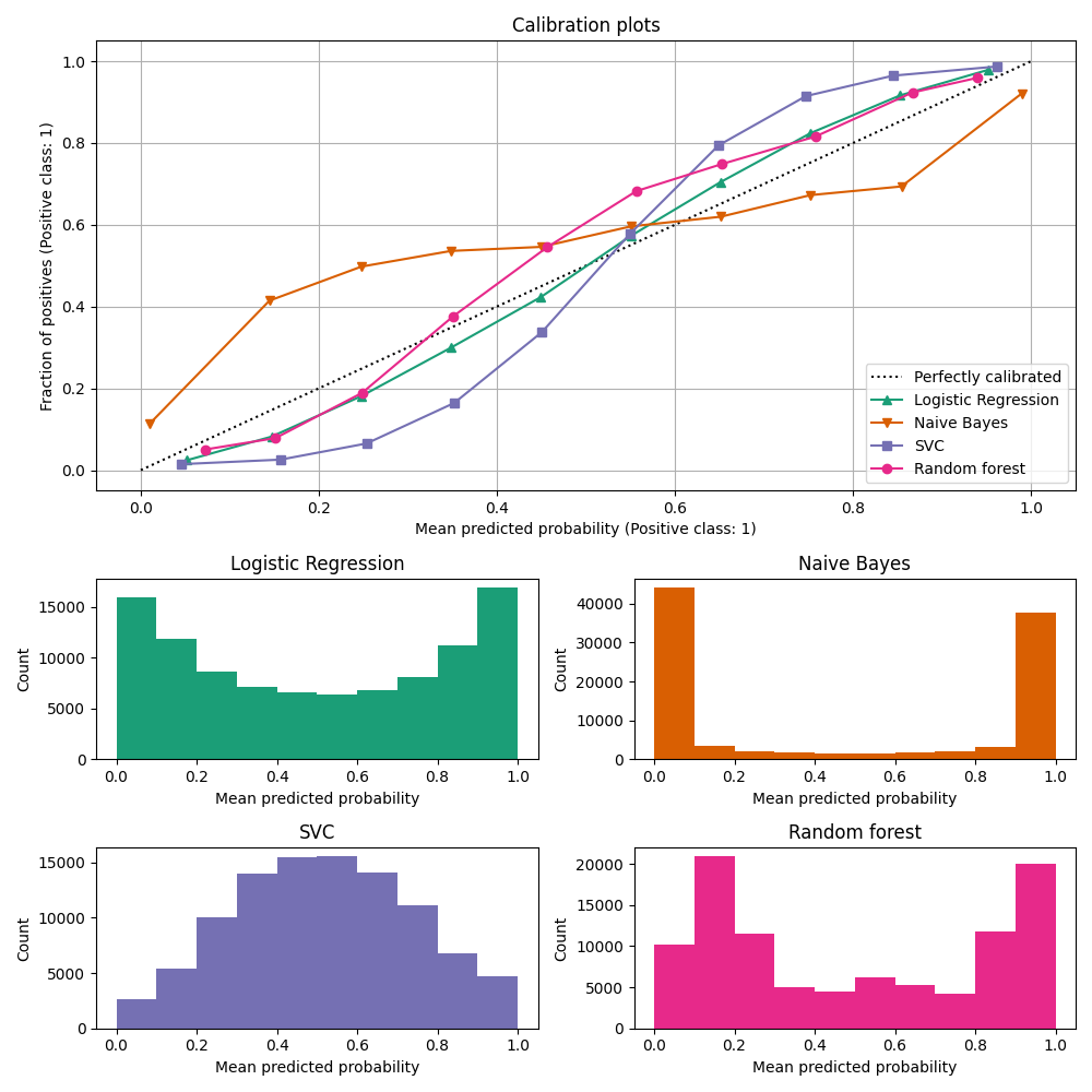
校准曲线

下面，我们使用小型训练数据集训练四个模型中的每一个，然后使用测试数据集的预测概率绘制校准曲线（也称为可靠性图）。校准曲线是通过对预测概率进行分类，然后根据观察到的频率（“阳性分数”）绘制每个分类中的平均预测概率来创建的。在校准曲线下方，我们绘制了一个显示预测概率的分布或更具体地说，显示每个预测概率箱中的样本数量的分布。

import numpy as np

from sklearn.svm import LinearSVC


class NaivelyCalibratedLinearSVC(LinearSVC):
    """LinearSVC with `predict_proba` method that naively scales
    `decision_function` output."""

    def fit(self, X, y):
        super().fit(X, y)
        df = self.decision_function(X)
        self.df_min_ = df.min()
        self.df_max_ = df.max()

    def predict_proba(self, X):
        """Min-max scale output of `decision_function` to [0,1]."""
        df = self.decision_function(X)
        calibrated_df = (df - self.df_min_) / (self.df_max_ - self.df_min_)
        proba_pos_class = np.clip(calibrated_df, 0, 1)
        proba_neg_class = 1 - proba_pos_class
        proba = np.c_[proba_neg_class, proba_pos_class]
        return proba

from sklearn.calibration import CalibrationDisplay
from sklearn.ensemble import RandomForestClassifier
from sklearn.linear_model import LogisticRegressionCV
from sklearn.naive_bayes import GaussianNB

# Define the classifiers to be compared in the study.
#
# Note that we use a variant of the logistic regression model that can
# automatically tune its regularization parameter.
#
# For a fair comparison, we should run a hyper-parameter search for all the
# classifiers but we don't do it here for the sake of keeping the example code
# concise and fast to execute.
lr = LogisticRegressionCV(
    Cs=np.logspace(-6, 6, 101), cv=10, scoring="neg_log_loss", max_iter=1_000
)
gnb = GaussianNB()
svc = NaivelyCalibratedLinearSVC(C=1.0)
rfc = RandomForestClassifier(random_state=42)

clf_list = [
    (lr, "Logistic Regression"),
    (gnb, "Naive Bayes"),
    (svc, "SVC"),
    (rfc, "Random forest"),
]

import matplotlib.pyplot as plt
from matplotlib.gridspec import GridSpec

fig = plt.figure(figsize=(10, 10))
gs = GridSpec(4, 2)
colors = plt.get_cmap("Dark2")

ax_calibration_curve = fig.add_subplot(gs[:2, :2])
calibration_displays = {}
markers = ["^", "v", "s", "o"]
for i, (clf, name) in enumerate(clf_list):
    clf.fit(X_train, y_train)
    display = CalibrationDisplay.from_estimator(
        clf,
        X_test,
        y_test,
        n_bins=10,
        name=name,
        ax=ax_calibration_curve,
        color=colors(i),
        marker=markers[i],
    )
    calibration_displays[name] = display

ax_calibration_curve.grid()
ax_calibration_curve.set_title("Calibration plots")

# Add histogram
grid_positions = [(2, 0), (2, 1), (3, 0), (3, 1)]
for i, (_, name) in enumerate(clf_list):
    row, col = grid_positions[i]
    ax = fig.add_subplot(gs[row, col])

    ax.hist(
        calibration_displays[name].y_prob,
        range=(0, 1),
        bins=10,
        label=name,
        color=colors(i),
    )
    ax.set(title=name, xlabel="Mean predicted probability", ylabel="Count")

plt.tight_layout()
plt.show()

结果分析

LogisticRegressionCV 尽管训练集大小很小，但仍返回相当良好的校准预测：其可靠性曲线是四个模型中最接近对角线的。

逻辑回归是通过最小化log损失来训练的，这是一个严格正确的评分规则：在无限训练数据的限制下，通过预测真实条件概率的模型最小化严格正确的评分规则。因此，该（假设的）模型将得到完美校准。然而，使用适当的评分规则作为训练目标并不足以保证模型本身经过良好校准：即使有非常大的训练集，逻辑回归仍然可能很差地校准，如果其规则化太强，或者输入要素的选择和预处理是否导致该模型指定错误（例如，如果数据集的真实决策边界是输入特征的高度非线性函数）。

在这个例子中，训练集故意保持非常小。在这种情况下，优化对数损失仍然可能导致模型由于过度匹配而校准不良。为了缓解这种情况， LogisticRegressionCV 类已配置为调整 C 正规化参数还可以通过内部交叉验证最小化日志损失，以便在小训练集设置中找到该模型的最佳妥协。

由于训练集大小有限并且缺乏良好规范的保证，我们观察到逻辑回归模型的校准曲线在对角线上很接近但并不完美。该模型的校准曲线的形状可以解释为略显自信不足：与阳性样本的真实分数相比，预测概率有点太接近0.5。

其他方法都输出不太好校准的概率：

• GaussianNB 倾向于将此特定数据集的概率推至0或1（参见图表）（过度自信）。这主要是因为朴素的Bayes方程只有在特征有条件独立的假设成立时才提供正确的概率估计 [2]. 然而，特征可以相互关联，这个数据集就是这种情况，它包含2个作为信息特征的随机线性组合生成的特征。这些相关特征实际上被“计数两次”，导致预测概率推向0和1 [3]. 然而，请注意，改变用于生成数据集的种子可能会导致朴素Bayes估计器的结果差异很大。

• LinearSVC 不是一个自然的概率分类器。为了如此解释其预测，我们天真地缩放了 decision_function 成 [0, 1] by applying min-max scaling in the NaivelyCalibratedLinearSVC wrapper class defined above. This estimator shows a typical sigmoid-shaped calibration curve on this data: predictions larger than 0.5 correspond to samples with an even larger effective positive class fraction (above the diagonal), while predictions below 0.5 corresponds to even lower positive class fractions (below the diagonal). This under-confident predictions are typical for maximum-margin methods [1] .

• RandomForestClassifier 的预测图表显示峰值在大约。0.2和0.9的概率，而接近0或1的概率非常罕见。对此的解释如下 [1]: “诸如装袋和随机森林等方法，对一组基本模型的预测进行平均，可能很难做出接近0和1的预测，因为基础基本模型的方差会使本应接近0或与这些值相差1的预测产生偏差。因为预测仅限于区间 [0, 1] ，方差引起的误差往往是单边的，接近零和一。例如，如果模型应该预测某个情况的p = 0，那么装袋实现这一目标的唯一方法是所有装袋树都预测为零。如果我们向装袋平均值的树木添加噪音，则这种噪音将导致一些树木在这种情况下预测大于0的值，从而将袋装集合的平均预测从0移开。我们在随机森林中观察到这种效果最强烈，因为使用随机森林训练的基础树由于特征子集设置而具有相对较高的方差。“这种效应可能会使随机森林缺乏信心。尽管存在这种可能的偏差，但请注意，树本身是通过最小化基尼或熵标准来进行匹配的，这两个标准都会导致最小化适当的评分规则的分裂：分别是Brier得分或log loss。看到 the user guide 了解更多详细信息。这可以解释为什么该模型在这个特定的示例数据集上显示了足够好的校准曲线。事实上，随机森林模型并不比逻辑回归模型明显更缺乏信心。

您可以使用不同的随机种子和其他数据集生成参数重新运行此示例，看看校准图看起来有多大不同。一般来说，逻辑回归和随机森林往往是最好的校准分类器，而SVC通常会显示典型的信心不足的误校准。朴素贝叶斯模型也经常校准不良，但其校准曲线的一般形状可能会因数据集而异。

最后，请注意，对于某些数据集种子，所有模型的校准都很差，即使如上所述调整正则化参数。当训练规模太小或模型被严重错误指定时，这必然会发生。

引用

[1] (1,2)

Predicting Good Probabilities with Supervised Learning <https://dl.acm.org/doi/pdf/10.1145/1102351.1102430> _，A。尼古列斯库-米齐尔& R.卡鲁阿纳，ICML 2005

[2]

Beyond independence: Conditions for the optimality of the simple bayesian classifier 多明戈斯，P.，&帕扎尼，M.，第13届国际会议会议。机器学习。1996.

[3]

Obtaining calibrated probability estimates from decision trees and naive Bayesian classifiers 扎德罗兹尼、比安卡和查尔斯·埃尔坎。Icml。第一卷。2001.

相关实例

概率校准曲线

Probability Calibration curves

分类器的概率校准

Probability calibration of classifiers

可视化VotingClassifier的概率预测

Visualizing the probabilistic predictions of a VotingClassifier

归纳集群

Inductive Clustering