使用概率PCA和因子分析（FA）进行模型选择#

概率PCA和因子分析都是概率模型。结果是，新数据的可能性可以用于模型选择和协方差估计。在这里，我们将PCA和FA与交叉验证进行了比较，这些数据被同方差噪音（每个特征的噪音方差相同）或异方差噪音（每个特征的噪音方差不同）破坏。在第二步中，我们将模型似然性与从收缩协方差估计器获得的似然性进行比较。

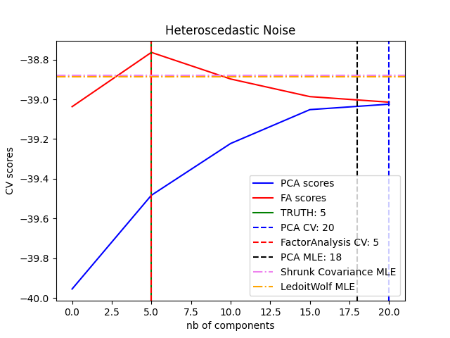
可以观察到，对于同方差噪音，FA和PCA都成功恢复了低阶子空间的大小。在这种情况下，PCA的可能性高于FA。然而，当存在异方差噪音时，PCA会失败并高估排名。在适当的情况下（选择组件数量），低等级模型比收缩模型更有可能使用持有数据。

PCA的随机性自动选择的自动估计。还比较了Thomas P. Minka的NIPS 2000：598-604。

# Authors: The scikit-learn developers
# SPDX-License-Identifier: BSD-3-Clause

创建数据#

import numpy as np
from scipy import linalg

n_samples, n_features, rank = 500, 25, 5
sigma = 1.0
rng = np.random.RandomState(42)
U, _, _ = linalg.svd(rng.randn(n_features, n_features))
X = np.dot(rng.randn(n_samples, rank), U[:, :rank].T)

# Adding homoscedastic noise
X_homo = X + sigma * rng.randn(n_samples, n_features)

# Adding heteroscedastic noise
sigmas = sigma * rng.rand(n_features) + sigma / 2.0
X_hetero = X + rng.randn(n_samples, n_features) * sigmas

适合模特#

import matplotlib.pyplot as plt

from sklearn.covariance import LedoitWolf, ShrunkCovariance
from sklearn.decomposition import PCA, FactorAnalysis
from sklearn.model_selection import GridSearchCV, cross_val_score

n_components = np.arange(0, n_features, 5)  # options for n_components


def compute_scores(X):
    pca = PCA(svd_solver="full")
    fa = FactorAnalysis()

    pca_scores, fa_scores = [], []
    for n in n_components:
        pca.n_components = n
        fa.n_components = n
        pca_scores.append(np.mean(cross_val_score(pca, X)))
        fa_scores.append(np.mean(cross_val_score(fa, X)))

    return pca_scores, fa_scores


def shrunk_cov_score(X):
    shrinkages = np.logspace(-2, 0, 30)
    cv = GridSearchCV(ShrunkCovariance(), {"shrinkage": shrinkages})
    return np.mean(cross_val_score(cv.fit(X).best_estimator_, X))


def lw_score(X):
    return np.mean(cross_val_score(LedoitWolf(), X))


for X, title in [(X_homo, "Homoscedastic Noise"), (X_hetero, "Heteroscedastic Noise")]:
    pca_scores, fa_scores = compute_scores(X)
    n_components_pca = n_components[np.argmax(pca_scores)]
    n_components_fa = n_components[np.argmax(fa_scores)]

    pca = PCA(svd_solver="full", n_components="mle")
    pca.fit(X)
    n_components_pca_mle = pca.n_components_

    print("best n_components by PCA CV = %d" % n_components_pca)
    print("best n_components by FactorAnalysis CV = %d" % n_components_fa)
    print("best n_components by PCA MLE = %d" % n_components_pca_mle)

    plt.figure()
    plt.plot(n_components, pca_scores, "b", label="PCA scores")
    plt.plot(n_components, fa_scores, "r", label="FA scores")
    plt.axvline(rank, color="g", label="TRUTH: %d" % rank, linestyle="-")
    plt.axvline(
        n_components_pca,
        color="b",
        label="PCA CV: %d" % n_components_pca,
        linestyle="--",
    )
    plt.axvline(
        n_components_fa,
        color="r",
        label="FactorAnalysis CV: %d" % n_components_fa,
        linestyle="--",
    )
    plt.axvline(
        n_components_pca_mle,
        color="k",
        label="PCA MLE: %d" % n_components_pca_mle,
        linestyle="--",
    )

    # compare with other covariance estimators
    plt.axhline(
        shrunk_cov_score(X),
        color="violet",
        label="Shrunk Covariance MLE",
        linestyle="-.",
    )
    plt.axhline(
        lw_score(X),
        color="orange",
        label="LedoitWolf MLE" % n_components_pca_mle,
        linestyle="-.",
    )

    plt.xlabel("nb of components")
    plt.ylabel("CV scores")
    plt.legend(loc="lower right")
    plt.title(title)

plt.show()

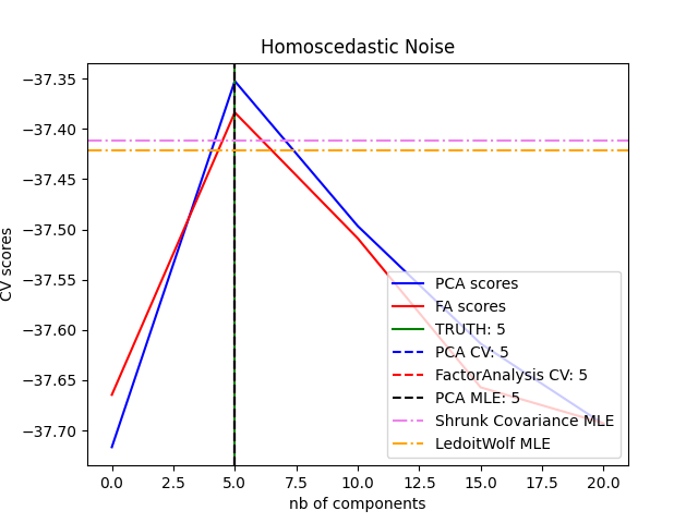
best n_components by PCA CV = 5
best n_components by FactorAnalysis CV = 5
best n_components by PCA MLE = 5
best n_components by PCA CV = 20
best n_components by FactorAnalysis CV = 5
best n_components by PCA MLE = 18

Total running time of the script: （0分3.735秒）