作为L2正则化函数的脊系数#

过度拟合的模型会很好地学习训练数据，捕获数据中的潜在模式和噪声。然而，当应用于看不见的数据时，学习的关联可能不成立。当我们将训练好的预测应用于测试数据时，我们通常会发现这一点，并看到与训练数据相比，统计性能显着下降。

克服过拟合的一种方法是通过正规化，这可以通过惩罚线性模型中的大权重（系数）来实现，迫使模型缩小所有系数。正规化减少了模型对从训练样本中获得的特定信息的依赖。

这个例子说明了如何在 Ridge 回归通过向随系数增加的损失添加惩罚项来影响模型的性能 \(\beta\) .

The regularized loss function is given by: \(\mathcal{L}(X, y, \beta) = \| y - X \beta \|^{2}_{2} + \alpha \| \beta \|^{2}_{2}\)

哪里 \(X\) 是输入数据， \(y\) 是目标变量， \(\beta\) 是与特征相关的系数的载体，并且 \(\alpha\) 就是正规化实力。

正规化损失函数旨在平衡准确预测训练集和防止过度匹配之间的权衡。

在这次常规化的损失中，左侧（例如 \(\|y - X\beta\|^{2}_{2}\) ）测量实际目标变量之间的平方差， \(y\) ，以及预测值。仅最小化这个项可能会导致过度逼近，因为模型可能会变得过于复杂且对训练数据中的噪音敏感。

To address overfitting, Ridge regularization adds a constraint, called a penalty term, (\(\alpha \| \beta\|^{2}_{2}\)) to the loss function. This penalty term is the sum of the squares of the model's coefficients, multiplied by the regularization strength \(\alpha\). By introducing this constraint, Ridge regularization discourages any single coefficient \(\beta_{i}\) from taking an excessively large value and encourages smaller and more evenly distributed coefficients. Higher values of \(\alpha\) force the coefficients towards zero. However, an excessively high \(\alpha\) can result in an underfit model that fails to capture important patterns in the data.

因此，正则化损失函数结合了预测精度项和惩罚项。通过调整正则化强度，从业者可以微调对权重施加的约束程度，训练一个能够很好地推广到不可见数据的模型，同时避免过度拟合。

# Authors: The scikit-learn developers
# SPDX-License-Identifier: BSD-3-Clause

这个例子的目的#

为了展示Ridge正规化的工作原理，我们将创建一个无噪数据集。然后我们将根据一系列正规化强度训练一个正规化模型 (\(\alpha\) ），并绘制训练后的系数以及这些系数与原始值之间的均方误差如何表现为正则化强度的函数。

创建无噪音数据集#

我们制作了一个包含100个样本和10个特征的玩具数据集，适合检测回归。在10个特征中，8个具有信息性并有助于回归，而其余2个特征对目标变量没有任何影响（其真实系数为0）。请注意，在这个示例中，数据是无噪的，因此我们可以期望我们的回归模型能够准确地恢复真实系数w。

from sklearn.datasets import make_regression

X, y, w = make_regression(
    n_samples=100, n_features=10, n_informative=8, coef=True, random_state=1
)

# Obtain the true coefficients
print(f"The true coefficient of this regression problem are:\n{w}")

The true coefficient of this regression problem are:
[38.32634568 88.49665188  0.         29.75747153  0.         19.08699432
 25.44381023 38.69892343 49.28808734 71.75949622]

训练山脊回归者#

我们使用 Ridge ，具有L2正规化的线性模型。我们训练多个模型，每个模型参数的值不同 alpha ，这是一个乘以罚项的正常数，控制规则化强度。然后，对于每个训练的模型，我们计算真实系数之间的误差 w 以及模型找到的系数 clf .我们将识别的系数和相应系数的计算误差存储在列表中，这使得我们可以方便地绘制它们。

import numpy as np

from sklearn.linear_model import Ridge
from sklearn.metrics import mean_squared_error

clf = Ridge()

# Generate values for `alpha` that are evenly distributed on a logarithmic scale
alphas = np.logspace(-3, 4, 200)
coefs = []
errors_coefs = []

# Train the model with different regularisation strengths
for a in alphas:
    clf.set_params(alpha=a).fit(X, y)
    coefs.append(clf.coef_)
    errors_coefs.append(mean_squared_error(clf.coef_, w))

绘制训练系数和均方误差#

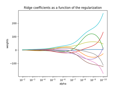
现在我们将10个不同的正规化系数绘制为正规化参数的函数 alpha 其中每种颜色表示不同的系数。

在右侧，我们绘制了估计器的系数误差如何作为正规化的函数而变化。

import matplotlib.pyplot as plt
import pandas as pd

alphas = pd.Index(alphas, name="alpha")
coefs = pd.DataFrame(coefs, index=alphas, columns=[f"Feature {i}" for i in range(10)])
errors = pd.Series(errors_coefs, index=alphas, name="Mean squared error")

fig, axs = plt.subplots(1, 2, figsize=(20, 6))

coefs.plot(
    ax=axs[0],
    logx=True,
    title="Ridge coefficients as a function of the regularization strength",
)
axs[0].set_ylabel("Ridge coefficient values")
errors.plot(
    ax=axs[1],
    logx=True,
    title="Coefficient error as a function of the regularization strength",
)
_ = axs[1].set_ylabel("Mean squared error")

Ridge coefficients as a function of the regularization strength, Coefficient error as a function of the regularization strength

解读情节#

左侧的图显示了规则化强度如何 (alpha ）影响岭回归系数。的较小值 alpha (weak正规化），允许系数与真实系数非常相似 (w ）用于生成数据集。这是因为没有向我们的人工数据集中添加额外的噪音。作为 alpha 增加时，系数会缩小为零，逐渐减少以前更重要的特征的影响。

右侧的图显示了模型得出的系数与真实系数之间的均方误差（MSE (w ).它提供了一种与我们的山脊模型与真正的生成模型相比的精确程度有关的测量。低误差意味着它找到的系数更接近真实生成模型的系数。在这种情况下，由于我们的玩具数据集是无噪的，因此我们可以看到最不正规化的模型检索最接近真实系数的系数 (w ）（错误接近0）。

当 alpha 由于模型很小，因此可以捕捉训练数据的复杂细节，无论这些细节是由噪音还是实际信息引起的。作为 alpha 增加时，最高系数缩小得更快，使其相应的特征在训练过程中的影响较小。这可以增强模型推广到不可见数据的能力（如果有很多噪音需要捕获），但如果与数据包含的噪音量相比，正规化变得太强，也会带来失去性能的风险（如本例中所示）。

在数据通常包括噪音的现实世界场景中，选择适当的 alpha 价值对于在过度适配和不足适配模型之间取得平衡至关重要。

在这里，我们看到 Ridge 对系数添加一个惩罚以对抗过度匹配。出现的另一个问题与训练数据集中异常值的存在有关。异常值是与其他观察结果显着不同的数据点。具体来说，这些异常值会影响我们之前展示的损失函数的左侧项。其他一些线性模型的制定对于离群值（例如 HuberRegressor .您可以在 HuberRegressor与Ridge在具有强异常值的数据集上 example.

Total running time of the script: （0分0.501秒）