多维标度#

生成的有噪数据上的指标和非指标BDS的说明。

# Authors: The scikit-learn developers
# SPDX-License-Identifier: BSD-3-Clause

数据集准备#

我们首先在2D空间中均匀生成20个点。

import numpy as np
from matplotlib import pyplot as plt
from matplotlib.collections import LineCollection

from sklearn import manifold
from sklearn.decomposition import PCA
from sklearn.metrics import euclidean_distances

# Generate the data
EPSILON = np.finfo(np.float32).eps
n_samples = 20
rng = np.random.RandomState(seed=3)
X_true = rng.randint(0, 20, 2 * n_samples).astype(float)
X_true = X_true.reshape((n_samples, 2))

# Center the data
X_true -= X_true.mean()

现在我们计算所有点之间的成对距离，并向距离矩阵添加少量噪音。我们确保保持有噪距离矩阵对称。

# Compute pairwise Euclidean distances
distances = euclidean_distances(X_true)

# Add noise to the distances
noise = rng.rand(n_samples, n_samples)
noise = noise + noise.T
np.fill_diagonal(noise, 0)
distances += noise

在这里，我们计算有噪距离矩阵的度量和非度量BDS。

mds = manifold.MDS(
    n_components=2,
    max_iter=3000,
    eps=1e-9,
    n_init=1,
    random_state=42,
    dissimilarity="precomputed",
    n_jobs=1,
)
X_mds = mds.fit(distances).embedding_

nmds = manifold.MDS(
    n_components=2,
    metric=False,
    max_iter=3000,
    eps=1e-12,
    dissimilarity="precomputed",
    random_state=42,
    n_jobs=1,
    n_init=1,
)
X_nmds = nmds.fit_transform(distances)

重新调整非度量SCS解决方案的比例以匹配原始数据的分布。

X_nmds *= np.sqrt((X_true**2).sum()) / np.sqrt((X_nmds**2).sum())

为了使视觉比较更容易，我们将原始数据和两个BDS解决方案旋转到它们的PCA轴。如果需要，可以翻转水平和垂直的BDS轴，以匹配原始数据方向。

# Rotate the data
pca = PCA(n_components=2)
X_true = pca.fit_transform(X_true)
X_mds = pca.fit_transform(X_mds)
X_nmds = pca.fit_transform(X_nmds)

# Align the sign of PCs
for i in [0, 1]:
    if np.corrcoef(X_mds[:, i], X_true[:, i])[0, 1] < 0:
        X_mds[:, i] *= -1
    if np.corrcoef(X_nmds[:, i], X_true[:, i])[0, 1] < 0:
        X_nmds[:, i] *= -1

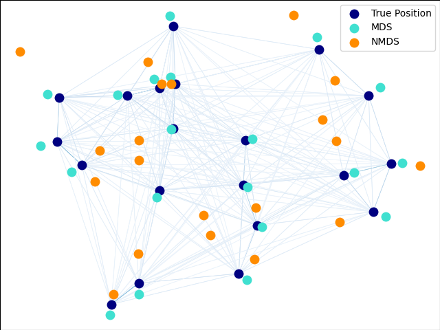
最后，我们绘制原始数据和两个BDS重建。

fig = plt.figure(1)
ax = plt.axes([0.0, 0.0, 1.0, 1.0])

s = 100
plt.scatter(X_true[:, 0], X_true[:, 1], color="navy", s=s, lw=0, label="True Position")
plt.scatter(X_mds[:, 0], X_mds[:, 1], color="turquoise", s=s, lw=0, label="MDS")
plt.scatter(X_nmds[:, 0], X_nmds[:, 1], color="darkorange", s=s, lw=0, label="NMDS")
plt.legend(scatterpoints=1, loc="best", shadow=False)

# Plot the edges
start_idx, end_idx = X_mds.nonzero()
# a sequence of (*line0*, *line1*, *line2*), where::
#            linen = (x0, y0), (x1, y1), ... (xm, ym)
segments = [
    [X_true[i, :], X_true[j, :]] for i in range(len(X_true)) for j in range(len(X_true))
]
edges = distances.max() / (distances + EPSILON) * 100
np.fill_diagonal(edges, 0)
edges = np.abs(edges)
lc = LineCollection(
    segments, zorder=0, cmap=plt.cm.Blues, norm=plt.Normalize(0, edges.max())
)
lc.set_array(edges.flatten())
lc.set_linewidths(np.full(len(segments), 0.5))
ax.add_collection(lc)

plt.show()

Total running time of the script: （0分0.110秒）