保序回归#

生成数据的等序回归的说明（非线性单调趋势和同向均匀噪音）。

等张回归算法找到函数的非递减逼近，同时最大限度地减少训练数据的均方误差。这种非参数模型的好处是，除了单调性之外，它不会为目标函数假设任何形状。为了进行比较，还提供了线性回归。

右侧的图显示了阈值点线性插值产生的模型预测函数。阈值点是训练输入观察的子集，其匹配目标值通过等张非参数匹配来计算。

# Authors: The scikit-learn developers
# SPDX-License-Identifier: BSD-3-Clause

import matplotlib.pyplot as plt
import numpy as np
from matplotlib.collections import LineCollection

from sklearn.isotonic import IsotonicRegression
from sklearn.linear_model import LinearRegression
from sklearn.utils import check_random_state

n = 100
x = np.arange(n)
rs = check_random_state(0)
y = rs.randint(-50, 50, size=(n,)) + 50.0 * np.log1p(np.arange(n))

适合IsotonicRegistry和Linear Registry模型：

ir = IsotonicRegression(out_of_bounds="clip")
y_ = ir.fit_transform(x, y)

lr = LinearRegression()
lr.fit(x[:, np.newaxis], y)  # x needs to be 2d for LinearRegression

LinearRegression()

In a Jupyter environment, please rerun this cell to show the HTML representation or trust the notebook.
On GitHub, the HTML representation is unable to render, please try loading this page with nbviewer.org.

情节结果：

segments = [[[i, y[i]], [i, y_[i]]] for i in range(n)]
lc = LineCollection(segments, zorder=0)
lc.set_array(np.ones(len(y)))
lc.set_linewidths(np.full(n, 0.5))

fig, (ax0, ax1) = plt.subplots(ncols=2, figsize=(12, 6))

ax0.plot(x, y, "C0.", markersize=12)
ax0.plot(x, y_, "C1.-", markersize=12)
ax0.plot(x, lr.predict(x[:, np.newaxis]), "C2-")
ax0.add_collection(lc)
ax0.legend(("Training data", "Isotonic fit", "Linear fit"), loc="lower right")
ax0.set_title("Isotonic regression fit on noisy data (n=%d)" % n)

x_test = np.linspace(-10, 110, 1000)
ax1.plot(x_test, ir.predict(x_test), "C1-")
ax1.plot(ir.X_thresholds_, ir.y_thresholds_, "C1.", markersize=12)
ax1.set_title("Prediction function (%d thresholds)" % len(ir.X_thresholds_))

plt.show()

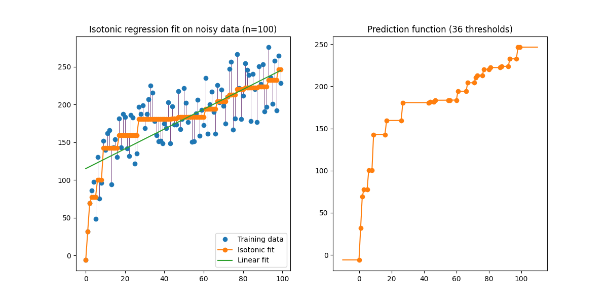
Isotonic regression fit on noisy data (n=100), Prediction function (36 thresholds)

请注意，我们明确通过了 out_of_bounds="clip" 致的构造者 IsotonicRegression 以控制模型在训练集中观察到的数据范围之外进行外推的方式。这种“削波”外推可以在右侧的决策函数图上看到。

Total running time of the script: （0分0.125秒）