核岭回归与SVR的比较#

核岭回归（KRR）和SVR都通过使用核技巧来学习非线性函数，即他们学习由相应核诱导的空间中的线性函数，该函数对应于原始空间中的非线性函数。它们在损失函数上有所不同（山脊与epsilon不敏感损失）。与SVR相比，KRR的匹配可以以封闭形式完成，并且对于中等规模的数据集通常更快。另一方面，学习到的模型是非稀疏的，因此在预测时比SVR慢。

此示例在人工数据集上展示了这两种方法，人工数据集由一个曲线目标函数和添加到每五个数据点的强噪音组成。

作者：scikit-learn开发人员SPDX-许可证-标识符：SD-3-Clause

生成示例数据#

import numpy as np

rng = np.random.RandomState(42)

X = 5 * rng.rand(10000, 1)
y = np.sin(X).ravel()

# Add noise to targets
y[::5] += 3 * (0.5 - rng.rand(X.shape[0] // 5))

X_plot = np.linspace(0, 5, 100000)[:, None]

构建基于核的回归模型#

from sklearn.kernel_ridge import KernelRidge
from sklearn.model_selection import GridSearchCV
from sklearn.svm import SVR

train_size = 100

svr = GridSearchCV(
    SVR(kernel="rbf", gamma=0.1),
    param_grid={"C": [1e0, 1e1, 1e2, 1e3], "gamma": np.logspace(-2, 2, 5)},
)

kr = GridSearchCV(
    KernelRidge(kernel="rbf", gamma=0.1),
    param_grid={"alpha": [1e0, 0.1, 1e-2, 1e-3], "gamma": np.logspace(-2, 2, 5)},
)

比较SVR和核岭回归的时间#

import time

t0 = time.time()
svr.fit(X[:train_size], y[:train_size])
svr_fit = time.time() - t0
print(f"Best SVR with params: {svr.best_params_} and R2 score: {svr.best_score_:.3f}")
print("SVR complexity and bandwidth selected and model fitted in %.3f s" % svr_fit)

t0 = time.time()
kr.fit(X[:train_size], y[:train_size])
kr_fit = time.time() - t0
print(f"Best KRR with params: {kr.best_params_} and R2 score: {kr.best_score_:.3f}")
print("KRR complexity and bandwidth selected and model fitted in %.3f s" % kr_fit)

sv_ratio = svr.best_estimator_.support_.shape[0] / train_size
print("Support vector ratio: %.3f" % sv_ratio)

t0 = time.time()
y_svr = svr.predict(X_plot)
svr_predict = time.time() - t0
print("SVR prediction for %d inputs in %.3f s" % (X_plot.shape[0], svr_predict))

t0 = time.time()
y_kr = kr.predict(X_plot)
kr_predict = time.time() - t0
print("KRR prediction for %d inputs in %.3f s" % (X_plot.shape[0], kr_predict))

Best SVR with params: {'C': 1.0, 'gamma': np.float64(0.1)} and R2 score: 0.737
SVR complexity and bandwidth selected and model fitted in 0.445 s
Best KRR with params: {'alpha': 0.1, 'gamma': np.float64(0.1)} and R2 score: 0.723
KRR complexity and bandwidth selected and model fitted in 0.166 s
Support vector ratio: 0.340
SVR prediction for 100000 inputs in 0.074 s
KRR prediction for 100000 inputs in 0.085 s

看结果#

import matplotlib.pyplot as plt

sv_ind = svr.best_estimator_.support_
plt.scatter(
    X[sv_ind],
    y[sv_ind],
    c="r",
    s=50,
    label="SVR support vectors",
    zorder=2,
    edgecolors=(0, 0, 0),
)
plt.scatter(X[:100], y[:100], c="k", label="data", zorder=1, edgecolors=(0, 0, 0))
plt.plot(
    X_plot,
    y_svr,
    c="r",
    label="SVR (fit: %.3fs, predict: %.3fs)" % (svr_fit, svr_predict),
)
plt.plot(
    X_plot, y_kr, c="g", label="KRR (fit: %.3fs, predict: %.3fs)" % (kr_fit, kr_predict)
)
plt.xlabel("data")
plt.ylabel("target")
plt.title("SVR versus Kernel Ridge")
_ = plt.legend()

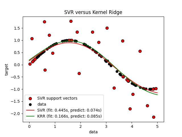
上图比较了当使用网格搜索优化RBS核的复杂性/正规化和带宽时KRR和SVR的学习模型。学习到的函数非常相似;然而，KRR的匹配速度大约比SVR快3-4倍（两者都使用网格搜索）。

理论上，使用SVR对100000个目标值的预测速度大约快三倍，因为它只使用大约1/3的训练数据点作为支持载体学习了稀疏模型。然而，在实践中，情况并不一定是这样，因为每个模型的核心函数计算方式的实现细节可以使KRR模型同样快甚至更快，尽管计算更多的算术运算。

可视化训练和预测时间#

plt.figure()

sizes = np.logspace(1, 3.8, 7).astype(int)
for name, estimator in {
    "KRR": KernelRidge(kernel="rbf", alpha=0.01, gamma=10),
    "SVR": SVR(kernel="rbf", C=1e2, gamma=10),
}.items():
    train_time = []
    test_time = []
    for train_test_size in sizes:
        t0 = time.time()
        estimator.fit(X[:train_test_size], y[:train_test_size])
        train_time.append(time.time() - t0)

        t0 = time.time()
        estimator.predict(X_plot[:1000])
        test_time.append(time.time() - t0)

    plt.plot(
        sizes,
        train_time,
        "o-",
        color="r" if name == "SVR" else "g",
        label="%s (train)" % name,
    )
    plt.plot(
        sizes,
        test_time,
        "o--",
        color="r" if name == "SVR" else "g",
        label="%s (test)" % name,
    )

plt.xscale("log")
plt.yscale("log")
plt.xlabel("Train size")
plt.ylabel("Time (seconds)")
plt.title("Execution Time")
_ = plt.legend(loc="best")

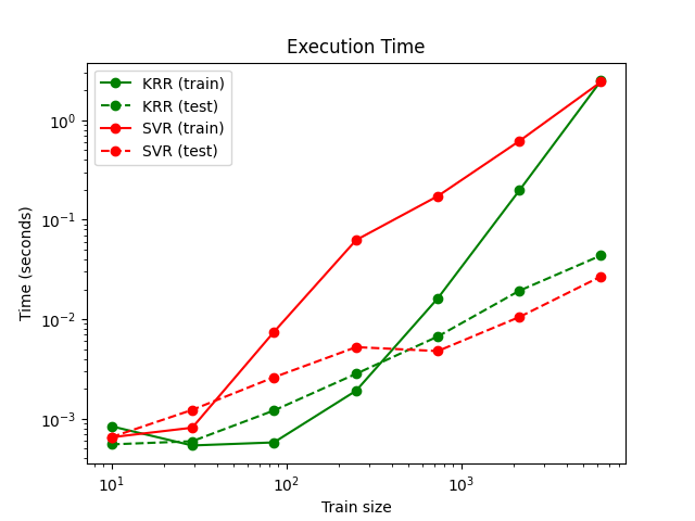
该图比较了不同大小训练集的KRR和SVR的匹配和预测时间。对于中等规模的训练集（少于几千个样本），KRR的匹配速度比SVR快;然而，对于较大的训练集，SVR的扩展性更好。关于预测时间，由于学习到的稀疏解，对于所有大小的训练集，SVR应该比KRR快，但由于实现细节，实际上情况不一定如此。请注意，稀疏度以及预测时间取决于SVR的参数RST和C。

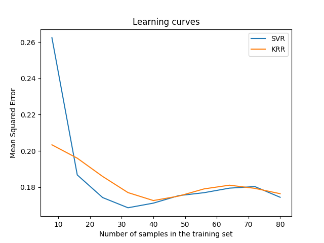
可视化学习曲线#

from sklearn.model_selection import LearningCurveDisplay

_, ax = plt.subplots()

svr = SVR(kernel="rbf", C=1e1, gamma=0.1)
kr = KernelRidge(kernel="rbf", alpha=0.1, gamma=0.1)

common_params = {
    "X": X[:100],
    "y": y[:100],
    "train_sizes": np.linspace(0.1, 1, 10),
    "scoring": "neg_mean_squared_error",
    "negate_score": True,
    "score_name": "Mean Squared Error",
    "score_type": "test",
    "std_display_style": None,
    "ax": ax,
}

LearningCurveDisplay.from_estimator(svr, **common_params)
LearningCurveDisplay.from_estimator(kr, **common_params)
ax.set_title("Learning curves")
ax.legend(handles=ax.get_legend_handles_labels()[0], labels=["SVR", "KRR"])

plt.show()

Total running time of the script: （0分7.485秒）