缩放SVCs的正规化参数#

The following example illustrates the effect of scaling the regularization parameter when using 支持向量机 for classification. For SVC classification, we are interested in a risk minimization for the equation:

\[C \sum_{i=1，n} \mathCal{L}（f（x_i），y_i）+ \Omega（w）\]

哪里

\(C\) 用于设置正规化量
\(\mathcal{L}\) 是一 loss 我们的样本和模型参数的函数。
\(\Omega\) 是一 penalty 我们的模型参数的函数

如果我们将损失函数视为每个样本的单个误差，那么数据匹配项或每个样本的误差总和会随着我们添加更多样本而增加。然而，处罚期限并没有增加。

例如，当使用时 cross validation ，设置规则化量 C ，交叉验证折叠内的主要问题和较小问题之间将存在不同数量的样本。

由于损失函数取决于样本数量，因此后者影响 C .出现的问题是“我们如何最佳地调整C以适应不同数量的训练样本？"

# Authors: The scikit-learn developers
# SPDX-License-Identifier: BSD-3-Clause

数据生成#

在本例中，我们研究重新参数化正规化参数的影响 C 以说明使用L1或L2罚分时的样本数量。为此目的，我们创建了一个具有大量特征的合成数据集，其中只有少数具有信息性。因此，我们期望正规化将系数缩小为零（L2罚分）或恰好为零（L1罚分）。

from sklearn.datasets import make_classification

n_samples, n_features = 100, 300
X, y = make_classification(
    n_samples=n_samples, n_features=n_features, n_informative=5, random_state=1
)

L1-处罚案例#

在L1的情况下，理论认为，由于提供了强的正规化，估计器无法像知道真实分布的模型一样进行预测（即使在样本量增长到无限大的限制下），因为它可能会将原本预测特征的一些权重设置为零，这会导致偏差。然而，它确实说，可以通过调整找到正确的非零参数集及其符号 C .

我们定义了一个线性SVC的L1惩罚。

from sklearn.svm import LinearSVC

model_l1 = LinearSVC(penalty="l1", loss="squared_hinge", dual=False, tol=1e-3)

我们计算不同值的平均测试分数 C 通过交叉验证。

import numpy as np
import pandas as pd

from sklearn.model_selection import ShuffleSplit, validation_curve

Cs = np.logspace(-2.3, -1.3, 10)
train_sizes = np.linspace(0.3, 0.7, 3)
labels = [f"fraction: {train_size}" for train_size in train_sizes]
shuffle_params = {
    "test_size": 0.3,
    "n_splits": 150,
    "random_state": 1,
}

results = {"C": Cs}
for label, train_size in zip(labels, train_sizes):
    cv = ShuffleSplit(train_size=train_size, **shuffle_params)
    train_scores, test_scores = validation_curve(
        model_l1,
        X,
        y,
        param_name="C",
        param_range=Cs,
        cv=cv,
        n_jobs=2,
    )
    results[label] = test_scores.mean(axis=1)
results = pd.DataFrame(results)

import matplotlib.pyplot as plt

fig, axes = plt.subplots(nrows=1, ncols=2, sharey=True, figsize=(12, 6))

# plot results without scaling C
results.plot(x="C", ax=axes[0], logx=True)
axes[0].set_ylabel("CV score")
axes[0].set_title("No scaling")

for label in labels:
    best_C = results.loc[results[label].idxmax(), "C"]
    axes[0].axvline(x=best_C, linestyle="--", color="grey", alpha=0.7)

# plot results by scaling C
for train_size_idx, label in enumerate(labels):
    train_size = train_sizes[train_size_idx]
    results_scaled = results[[label]].assign(
        C_scaled=Cs * float(n_samples * np.sqrt(train_size))
    )
    results_scaled.plot(x="C_scaled", ax=axes[1], logx=True, label=label)
    best_C_scaled = results_scaled["C_scaled"].loc[results[label].idxmax()]
    axes[1].axvline(x=best_C_scaled, linestyle="--", color="grey", alpha=0.7)

axes[1].set_title("Scaling C by sqrt(1 / n_samples)")

_ = fig.suptitle("Effect of scaling C with L1 penalty")

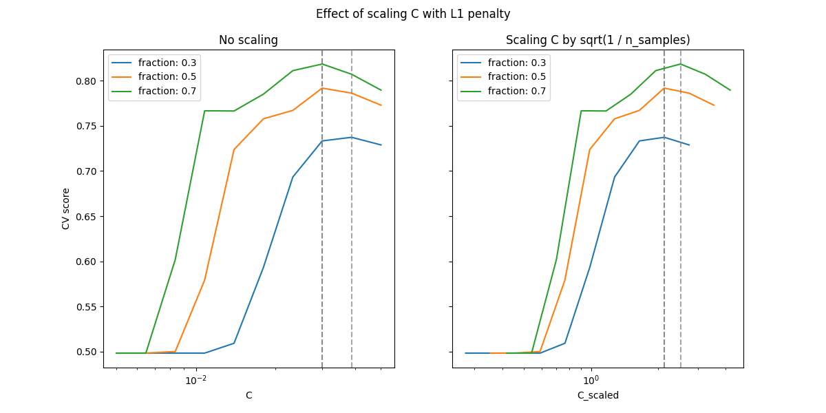
Effect of scaling C with L1 penalty, No scaling, Scaling C by sqrt(1 / n_samples)

在小地区 C （强正规化）模型学习的所有系数都为零，导致严重的欠拟。事实上，该地区的准确性处于偶然水平。

使用默认比例会产生比较稳定的最佳值 C ，而脱离欠匹配区域的转变取决于训练样本的数量。重新参数化会带来更稳定的结果。

参见例如的定理3 On the prediction performance of the Lasso 或 Simultaneous analysis of Lasso and Dantzig selector 其中，正则化参数总是被假定为与1 / sqrt（n_samples）成比例。

L2-处罚案例#

我们可以用L2罚分做类似的实验。在这种情况下，该理论认为，为了实现预测一致性，惩罚参数应该随着样本数量的增加而保持恒定。

model_l2 = LinearSVC(penalty="l2", loss="squared_hinge", dual=True)
Cs = np.logspace(-8, 4, 11)

labels = [f"fraction: {train_size}" for train_size in train_sizes]
results = {"C": Cs}
for label, train_size in zip(labels, train_sizes):
    cv = ShuffleSplit(train_size=train_size, **shuffle_params)
    train_scores, test_scores = validation_curve(
        model_l2,
        X,
        y,
        param_name="C",
        param_range=Cs,
        cv=cv,
        n_jobs=2,
    )
    results[label] = test_scores.mean(axis=1)
results = pd.DataFrame(results)

import matplotlib.pyplot as plt

fig, axes = plt.subplots(nrows=1, ncols=2, sharey=True, figsize=(12, 6))

# plot results without scaling C
results.plot(x="C", ax=axes[0], logx=True)
axes[0].set_ylabel("CV score")
axes[0].set_title("No scaling")

for label in labels:
    best_C = results.loc[results[label].idxmax(), "C"]
    axes[0].axvline(x=best_C, linestyle="--", color="grey", alpha=0.8)

# plot results by scaling C
for train_size_idx, label in enumerate(labels):
    results_scaled = results[[label]].assign(
        C_scaled=Cs * float(n_samples * np.sqrt(train_sizes[train_size_idx]))
    )
    results_scaled.plot(x="C_scaled", ax=axes[1], logx=True, label=label)
    best_C_scaled = results_scaled["C_scaled"].loc[results[label].idxmax()]
    axes[1].axvline(x=best_C_scaled, linestyle="--", color="grey", alpha=0.8)
axes[1].set_title("Scaling C by sqrt(1 / n_samples)")

fig.suptitle("Effect of scaling C with L2 penalty")
plt.show()

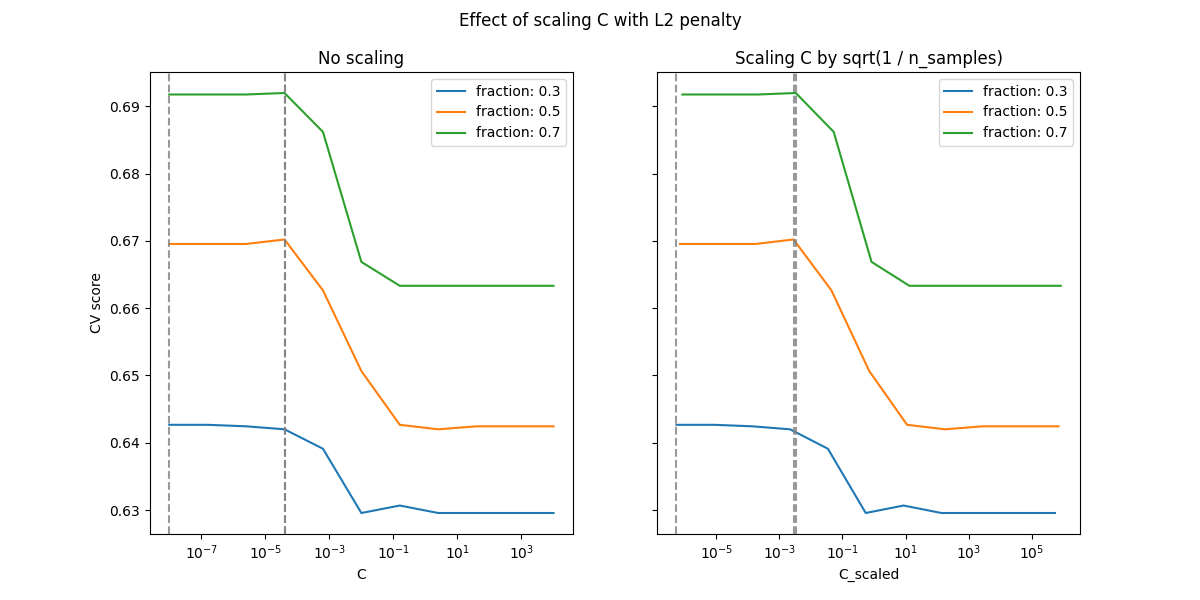
Effect of scaling C with L2 penalty, No scaling, Scaling C by sqrt(1 / n_samples)

对于L2罚情况，重新参数化似乎对正规化最佳值的稳定性影响较小。过度匹配区域的转变发生在更广泛的范围内，并且准确性似乎不会下降到机会水平。

尝试增加值， n_splits=1_000 以获得更好的L2情况下的结果，由于文档构建器的限制，这里没有显示。

Total running time of the script: (0 minutes 19.262 seconds)