1.4. 支持向量机

Support vector machines (SVMs) 是一套监督学习方法，用于 classification , regression 和 outliers detection .

支持向量机的优点是：

• 在多维空间中有效。

• 在维度数量大于样本数量的情况下仍然有效。

• 在决策函数中使用训练点的子集（称为支持载体），因此它也具有内存效率。

• 多才多艺：不同 核函数 可以为决策功能指定。提供了通用内核，但也可以指定自定义内核。

支持向量机的缺点包括：

• 如果要素数量远大于样本数量，则避免选择时过度适合 核函数 而正规化期限至关重要。

• SVMs不直接提供概率估计，这些估计是使用昂贵的五重交叉验证计算的（请参阅 Scores and probabilities ，下面）。

scikit-learn中的支持载体机支持密集型 (numpy.ndarray 并通过以下方式转换为 numpy.asarray ）和稀疏（任何 scipy.sparse ）样本载体作为输入。然而，要使用支持机对稀疏数据进行预测，它必须适合此类数据。为了获得最佳性能，请使用C排序 numpy.ndarray （密集）或 scipy.sparse.csr_matrix （sparse）with dtype=float64 .

1.4.1. 分类

SVC , NuSVC 和 LinearSVC 是能够对数据集执行二进制和多类分类的类。

SVC 和 NuSVC 方法相似，但接受略有不同的参数集并具有不同的数学公式（请参阅部分 数学公式 ).另一方面， LinearSVC 是线性核情况下支持向量分类的另一种（更快）实现。它还缺乏一些属性 SVC 和 NuSVC ，就像 support_ . LinearSVC 使用 squared_hinge 损失以及由于其实施 liblinear 如果考虑的话，它还可以规范拦截。然而，可以通过仔细微调其 intercept_scaling 参数，它允许拦截项具有与其他特征相比不同的规则化行为。因此，分类结果和分数可能与其他两个分类器不同。

与其他分类器一样， SVC , NuSVC 和 LinearSVC 将两个数组作为输入：一个数组 X 形状 (n_samples, n_features) 保存训练样本和阵列 y 类标签（字符串或integer）、形状 (n_samples)

>>> from sklearn import svm
>>> X = [[0, 0], [1, 1]]
>>> y = [0, 1]
>>> clf = svm.SVC()
>>> clf.fit(X, y)
SVC()

匹配后，模型可用于预测新值：：

>>> clf.predict([[2., 2.]])
array([1])

SVMs决策功能（详细信息请参阅 数学公式 ）取决于训练数据的某个子集，称为支持载体。这些支持载体的一些属性可以在属性中找到 support_vectors_ , support_ 和 n_support_

>>> # get support vectors
>>> clf.support_vectors_
array([[0., 0.],
       [1., 1.]])
>>> # get indices of support vectors
>>> clf.support_
array([0, 1]...)
>>> # get number of support vectors for each class
>>> clf.n_support_
array([1, 1]...)

示例

• SV：最大裕度分离超平面

• SVM-Anova：具有单变量特征选择的支持者

• sphx_glr_auto_examples_classification_plot_classification_probability.py

1.4.1.1. 多类分类

SVC 和 NuSVC 实施多类别分类的“一对一”方法。总的来说， n_classes * (n_classes - 1) / 2 构建分类器，每个分类器训练来自两个类别的数据。为了提供与其他分类器的一致界面， decision_function_shape 选项允许将“一对一”分类器的结果单调地转换为形状的“一对一”决策函数 (n_samples, n_classes) ，这是参数的默认设置（默认=' ovr '）。

>>> X = [[0], [1], [2], [3]]
>>> Y = [0, 1, 2, 3]
>>> clf = svm.SVC(decision_function_shape='ovo')
>>> clf.fit(X, Y)
SVC(decision_function_shape='ovo')
>>> dec = clf.decision_function([[1]])
>>> dec.shape[1] # 6 classes: 4*3/2 = 6
6
>>> clf.decision_function_shape = "ovr"
>>> dec = clf.decision_function([[1]])
>>> dec.shape[1] # 4 classes
4

另一方面， LinearSVC 实施“一对一”的多班策略，从而进行培训 n_classes 模型

>>> lin_clf = svm.LinearSVC()
>>> lin_clf.fit(X, Y)
LinearSVC()
>>> dec = lin_clf.decision_function([[1]])
>>> dec.shape[1]
4

看到 数学公式 获取决策功能的完整描述。

多类别策略的详细信息

注意到 LinearSVC 还实现了另一种多类策略，即Crammer和Singer制定的所谓多类支持者 [16], 通过使用该选项 multi_class='crammer_singer' .在实践中，通常首选一对休息分类，因为结果大多相似，但运行时间明显较少。

对于“一对休息” LinearSVC 的属性 coef_ 和 intercept_ 使形状 (n_classes, n_features) 和 (n_classes,) 分别系数的每一行对应于 n_classes “一vs-rest”分类器和拦截的类似分类器，按照“一”类的顺序。

在“一对一”的情况下 SVC 和 NuSVC ，属性的布局稍微复杂一些。对于线性内核，属性 coef_ 和 intercept_ 使形状 (n_classes * (n_classes - 1) / 2, n_features) 和 (n_classes * (n_classes - 1) / 2) 分别这类似于 LinearSVC 如上所述，每一行现在对应于二进制分类器。类0到n的顺序是“0 vs 1”、“0 vs 2”、.“0 vs n”、“1 vs 2”、“1 vs 3”、“1 vs n”、。. .“n-1 vs n”。

The shape of dual_coef_ is (n_classes-1, n_SV) with a somewhat hard to grasp layout. The columns correspond to the support vectors involved in any of the n_classes * (n_classes - 1) / 2 "one-vs-one" classifiers. Each support vector v has a dual coefficient in each of the n_classes - 1 classifiers comparing the class of v against another class. Note that some, but not all, of these dual coefficients, may be zero. The n_classes - 1 entries in each column are these dual coefficients, ordered by the opposing class.

这可能通过一个例子会更清楚：考虑一个三类问题，其中0类具有三个支持载体 \(v^{0}_0, v^{1}_0, v^{2}_0\) 并且第1类和第2类具有两个支持载体 \(v^{0}_1, v^{1}_1\) 和 \(v^{0}_2, v^{1}_2\) 分别 对于每个支持载体 \(v^{j}_i\) ，有两个双重系数。 让我们称支持量的系数 \(v^{j}_i\) 在类之间的分类器中 \(i\) 和 \(k\) \(\alpha^{j}_{i,k}\) .然后 dual_coef_ 看起来像这样：

\(\alpha^{0}_{0,1}\)	\(\alpha^{1}_{0,1}\)	\(\alpha^{2}_{0,1}\)	\(\alpha^{0}_{1,0}\)	\(\alpha^{1}_{1,0}\)	\(\alpha^{0}_{2,0}\)	\(\alpha^{1}_{2,0}\)
\(\alpha^{0}_{0,2}\)	\(\alpha^{1}_{0,2}\)	\(\alpha^{2}_{0,2}\)	\(\alpha^{0}_{1,2}\)	\(\alpha^{1}_{1,2}\)	\(\alpha^{0}_{2,1}\)	\(\alpha^{1}_{2,1}\)
0类SV的系数			1级SV的系数		2类SV的系数

示例

• 在虹膜数据集中绘制不同的支持者分类器

1.4.1.2. 分数和概率

的 decision_function 方法 SVC 和 NuSVC 为每个样本提供每个类别的分数（或在二进制情况下为每个样本提供单个分数）。当构造函数选项 probability 设置为 True 、类成员资格概率估计（来自方法 predict_proba 和 predict_log_proba ）已启用。在二进制的情况下，使用Platt标度来校准概率 [9]: 对支持者得分进行逻辑回归，通过对训练数据进行额外的交叉验证进行匹配。在多类情况下，这将根据 [10].

备注

通过 CalibratedClassifierCV （见 概率定标 ).的情况下 SVC 和 NuSVC ，此过程旨在 libsvm 它是在引擎盖下使用的，所以它不依赖于scikit-learn的 CalibratedClassifierCV .

Platt缩放涉及的交叉验证对于大型数据集来说是一项昂贵的操作。此外，概率估计可能与分数不一致：

• 分数的“argmax”可能不是概率的argmax

• 在二进制分类中，样本可以被标记为 predict 即使的输出，也属于正类 predict_proba 小于0.5;同样，即使的输出，它也可以被标记为负 predict_proba 大于0.5。

众所周知，普拉特的方法也存在理论问题。如果需要置信度分数，但这些不一定是概率，那么建议设置 probability=False 和使用 decision_function 而不是 predict_proba .

请注意，当 decision_function_shape='ovr' 和 n_classes > 2 ，不像 decision_function ， predict 默认情况下，方法不会尝试打破联系。您可以设置 break_ties=True 用于输出 predict 为相同 np.argmax(clf.decision_function(...), axis=1) ，否则绑定类中的第一个类将始终返回;但请记住，它会带来计算成本。看到 SV打破平局示例 以打破平局的例子。

1.4.1.3. 不平衡的问题

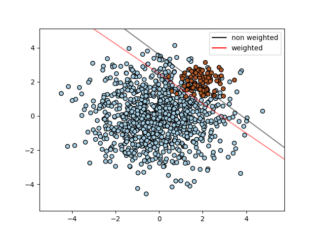
在希望更加重视某些类别或某些单个样本的问题中，参数 class_weight 和 sample_weight 可以使用

SVC (but不 NuSVC ）实现参数 class_weight 在 fit 法这是一本字典 {class_label : value} ，其中值是设置参数的> 0的浮点数 C 类 class_label 到 C * value .下图说明了不平衡问题的决策边界，有和没有权重修正。

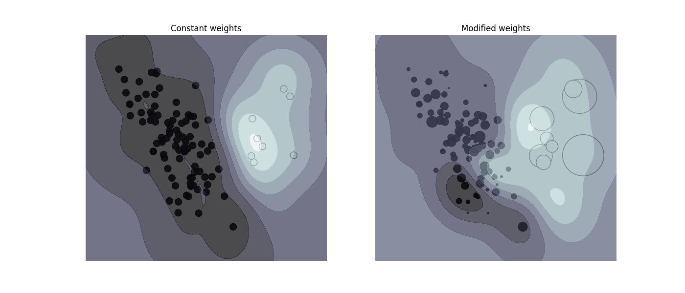
SVC, NuSVC, SVR, NuSVR, LinearSVC, LinearSVR and OneClassSVM implement also weights for individual samples in the fit method through the sample_weight parameter. Similar to class_weight, this sets the parameter C for the i-th example to C * sample_weight[i], which will encourage the classifier to get these samples right. The figure below illustrates the effect of sample weighting on the decision boundary. The size of the circles is proportional to the sample weights:

示例

• 支持者：分离不平衡类别的超平面

• 支持者：加权样本

1.4.2. 回归

支持向量分类方法可以扩展来解决回归问题。这种方法称为支持向量回归。

支持向量分类（如上所述）产生的模型仅取决于训练数据的子集，因为构建模型的成本函数并不关心超出边界的训练点。类似地，支持向量回归生成的模型仅取决于训练数据的一个子集，因为成本函数忽略了预测接近目标的样本。

支持量回归有三种不同的实现： SVR , NuSVR 和 LinearSVR . LinearSVR 提供比 SVR 但只考虑线性核，而 NuSVR 实施的公式与 SVR 和 LinearSVR .由于其实施于 liblinear LinearSVR 如果考虑的话，还可以规范拦截。然而，可以通过仔细微调其 intercept_scaling 参数，它允许拦截项具有与其他特征相比不同的规则化行为。因此，分类结果和分数可能与其他两个分类器不同。看到 实现细节 了解详情。

与分类类一样，fit方法将采用参数载体X、y，只是在这种情况下，y预计具有浮点值而不是整值：：

>>> from sklearn import svm
>>> X = [[0, 0], [2, 2]]
>>> y = [0.5, 2.5]
>>> regr = svm.SVR()
>>> regr.fit(X, y)
SVR()
>>> regr.predict([[1, 1]])
array([1.5])

示例

• 使用线性和非线性核的支持量回归（SVR）

1.4.3. 密度估计、新奇检测

类 OneClassSVM 实现一个用于异常值检测的单类支持者。

看到 新颖性和异常值检测 了解OneClassSV的描述和使用。

1.4.4. 复杂性

支持向量机是功能强大的工具，但它们的计算和存储需求随着训练向量的增加而迅速增加。支持者的核心是二次规划问题（QP），将支持载体与其余训练数据分离。使用的QP解算器 libsvm - 基于实施的范围介于 \(O(n_{features} \times n_{samples}^2)\) 和 \(O(n_{features} \times n_{samples}^3)\) 取决于 libsvm 实践中使用缓存（取决于数据集）。如果数据非常稀疏 \(n_{features}\) 应该被样本载体中非零特征的平均数量替换。

对于线性情况，使用的算法 LinearSVC 由 liblinear 实施比它的高效得多 libsvm - 基于 SVC 对应的，并且几乎可以线性扩展到数百万个样本和/或特征。

1.4.5. 实际使用技巧

• Avoiding data copy ：对于 SVC , SVR , NuSVC 和 NuSVR ，如果传递给某些方法的数据不是C排序连续和双精度，则在调用底层C实现之前将对其进行复制。您可以通过检查给定的numpy数组是否C连续 flags 属性

  为 LinearSVC （和 LogisticRegression ）任何作为numpy数组传递的输入都将被复制并转换到 liblinear 内部稀疏数据表示（双精度浮点数和非零分量的int 32索引）。如果您想适应大规模线性分类器，而不复制密集的麻木C连续双精度数组作为输入，我们建议使用 SGDClassifier 相反，班级。 目标函数可以配置为几乎与 LinearSVC 模型

• Kernel cache size ：对于 SVC , SVR , NuSVC 和 NuSVR ，内核缓存的大小对较大问题的运行时间有很大影响。 如果您有足够的RAM可用，建议设置 cache_size 设置为比默认值200（MB）更高的值，例如500（MB）或1000（MB）。

• Setting C : C 是 1 默认情况下，这是一个合理的默认选择。 如果您有很多有噪音的观察，您应该减少它：减少C对应于更多的正规化。

  LinearSVC 和 LinearSVR 不太敏感 C 当它变大，并且预测结果在一定阈值后停止改善时。与此同时，更大 C 值需要更多时间来训练，有时长达10倍，如所示 [11].

• 支持向量机算法不是规模不变的，因此 it is highly recommended to scale your data .例如，将输入载体X上的每个属性缩放为 [0,1] 或 [-1,+1] ，或将其标准化以使其均值为0和方差为1。注意到 same 必须将缩放应用于测试载体才能获得有意义的结果。通过使用 Pipeline

  >>> from sklearn.pipeline import make_pipeline
  >>> from sklearn.preprocessing import StandardScaler
  >>> from sklearn.svm import SVC
  
  >>> clf = make_pipeline(StandardScaler(), SVC())
  

  见章节 预处理数据 了解有关扩展和规范化的更多详细信息。

• Regarding the shrinking parameter, quoting [12]: We found that if the number of iterations is large, then shrinking can shorten the training time. However, if we loosely solve the optimization problem (e.g., by using a large stopping tolerance), the code without using shrinking may be much faster

• 参数 nu 在 NuSVC/OneClassSVM /：Class：“NuSVR”接近训练错误和支持载体的比例。

• 在 SVC ，如果数据不平衡（例如，多为正值，少为负值），则设置 class_weight='balanced' 和/或尝试不同的惩罚参数 C .

• Randomness of the underlying implementations: The underlying implementations of SVC and NuSVC use a random number generator only to shuffle the data for probability estimation (when probability is set to True). This randomness can be controlled with the random_state parameter. If probability is set to False these estimators are not random and random_state has no effect on the results. The underlying OneClassSVM implementation is similar to the ones of SVC and NuSVC. As no probability estimation is provided for OneClassSVM, it is not random.

  底层 LinearSVC 当用双坐标下降来匹配模型时（即，当 dual 设置为 True ).因此，相同输入数据的结果略有不同的情况并不罕见。如果发生这种情况，请尝试使用较小的 tol 参数.这种随机性也可以通过 random_state 参数.当 dual 设置为 False 的底层实现 LinearSVC 不是随机的， random_state 对结果没有影响。

• 使用由提供的L1处罚 LinearSVC(penalty='l1', dual=False) 产生稀疏解，即只有特征权重的子集不同于零并对决策函数有贡献。增加 C 产生更复杂的模型（选择更多特征）。的 C 产生“空”模型（所有权重均等于零）的值可以使用以下公式计算 l1_min_c .

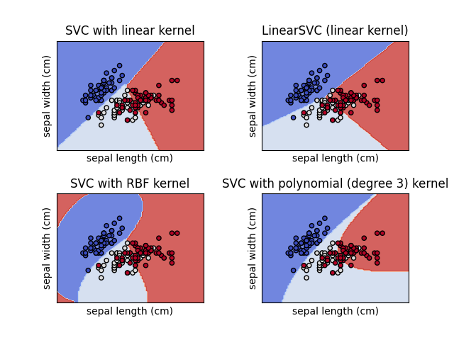
1.4.6. 核函数

的 kernel function 可以是以下任何一种：

• 线性： \(\langle x, x'\rangle\) .

• 多项： \((\gamma \langle x, x'\rangle + r)^d\) ，在哪里 \(d\) 由参数指定 degree , \(r\) 通过 coef0 .

• rbf: \(\exp(-\gamma \|x-x'\|^2)\), where \(\gamma\) is specified by parameter gamma, must be greater than 0.

• sigmoid \(\tanh(\gamma \langle x,x'\rangle + r)\), where \(r\) is specified by coef0.

不同的内核由 kernel 参数：：

>>> linear_svc = svm.SVC(kernel='linear')
>>> linear_svc.kernel
'linear'
>>> rbf_svc = svm.SVC(kernel='rbf')
>>> rbf_svc.kernel
'rbf'

另见 核近似 使用RBF内核的解决方案更快，更具可扩展性。

1.4.6.1. RBS核参数

当使用训练支持机时 Radial Basis Function (RBF)内核，必须考虑两个参数： C 和 gamma . 参数 C ，共同的所有支持向量机内核，权衡错误分类的训练样本对简单的决策表面。低 C 使决策表面光滑，同时高 C 旨在正确分类所有训练示例。 gamma 定义单个训练示例具有多大影响力。越大 gamma 是，其他例子必须受到影响得越近。

适当选择 C 和 gamma 对于支持机的性能至关重要。 建议使用 GridSearchCV 与 C 和 gamma 以指数级距离间隔以选择良好的价值观。

示例

• RBF SVM参数

• 缩放SVCs的正规化参数

1.4.6.2. 定制核

您可以通过将内核作为Python函数或通过预计算Gram矩阵来定义自己的内核。

具有自定义内核的分类器与任何其他分类器的行为相同，除了：

• 领域 support_vectors_ 现在为空，仅存储支持量的索引 support_

• 中第一个参数的引用（而不是副本） fit() 方法被存储以供将来参考。如果该数组在使用 fit() 和 predict() 你会得到意想不到的结果。

使用Python函数作为核心

您可以通过将函数传递给 kernel 参数.

Your kernel must take as arguments two matrices of shape (n_samples_1, n_features), (n_samples_2, n_features) and return a kernel matrix of shape (n_samples_1, n_samples_2).

以下代码定义线性内核并创建将使用该内核的分类器实例：：

>>> import numpy as np
>>> from sklearn import svm
>>> def my_kernel(X, Y):
...     return np.dot(X, Y.T)
...
>>> clf = svm.SVC(kernel=my_kernel)

使用克兰矩阵

您可以通过使用 kernel='precomputed' 选项.然后您应该将Gram矩阵而不是X传递给 fit 和 predict 方法.之间的内核值 all 必须提供训练载体和测试载体：

>>> import numpy as np
>>> from sklearn.datasets import make_classification
>>> from sklearn.model_selection import train_test_split
>>> from sklearn import svm
>>> X, y = make_classification(n_samples=10, random_state=0)
>>> X_train , X_test , y_train, y_test = train_test_split(X, y, random_state=0)
>>> clf = svm.SVC(kernel='precomputed')
>>> # linear kernel computation
>>> gram_train = np.dot(X_train, X_train.T)
>>> clf.fit(gram_train, y_train)
SVC(kernel='precomputed')
>>> # predict on training examples
>>> gram_test = np.dot(X_test, X_train.T)
>>> clf.predict(gram_test)
array([0, 1, 0])

示例

• 具有自定义内核的支持者

1.4.7. 数学公式

支持向量机在高维或无限维空间中构建一个超平面或一组超平面，可用于分类、回归或其他任务。直观地说，与任何类别的最近训练数据点距离最大的超平面（所谓的功能裕度）可以实现良好的分离，因为一般来说，裕度越大，分类器的概括误差就越低。下图显示了线性可分问题的决策函数，其中边界上有三个样本，称为“支持载体”：

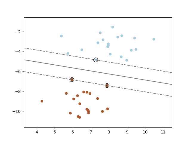
一般来说，当问题不可线性分离时，支持载体就是样本 within 边缘边界。

我们建议 [13] 和 [14] 作为支持者支持机的理论和实践的良好参考。

1.4.7.1. SVC

Given training vectors \(x_i \in \mathbb{R}^p\), i=1,..., n, in two classes, and a vector \(y \in \{1, -1\}^n\), our goal is to find \(w \in \mathbb{R}^p\) and \(b \in \mathbb{R}\) such that the prediction given by \(\text{sign} (w^T\phi(x) + b)\) is correct for most samples.

SRC解决了以下主要问题：

\[ \begin{align}\begin{aligned}\min_ {w, b, \zeta} \frac{1}{2} w^T w + C \sum_{i=1}^{n} \zeta_i\\\begin{split}\textrm {subject to } & y_i (w^T \phi (x_i) + b) \geq 1 - \zeta_i,\\ & \zeta_i \geq 0, i=1, ..., n\end{split}\end{aligned}\end{align} \]

直觉上，我们正在试图最大化利润（通过最小化 \(||w||^2 = w^Tw\) ），而当样本被错误分类或在边缘边界内时，则会产生处罚。理想情况下，价值 \(y_i (w^T \phi (x_i) + b)\) 将是 \(\geq 1\) 对于所有样本，这表明完美的预测。但问题通常并不总是与超平面完全分离，因此我们允许一些样本在一定距离处 \(\zeta_i\) 从正确的边缘边界开始。处罚期限 C 控制此惩罚的强度，因此充当逆正规化参数（见下文注释）。

原始的双重问题是

\[ \begin{align}\begin{aligned}\min_{\alpha} \frac{1}{2} \alpha^T Q \alpha - e^T \alpha\\\begin{split} \textrm {subject to } & y^T \alpha = 0\\ & 0 \leq \alpha_i \leq C, i=1, ..., n\end{split}\end{aligned}\end{align} \]

where \(e\) is the vector of all ones, and \(Q\) is an \(n\) by \(n\) positive semidefinite matrix, \(Q_{ij} \equiv y_i y_j K(x_i, x_j)\), where \(K(x_i, x_j) = \phi (x_i)^T \phi (x_j)\) is the kernel. The terms \(\alpha_i\) are called the dual coefficients, and they are upper-bounded by \(C\). This dual representation highlights the fact that training vectors are implicitly mapped into a higher (maybe infinite) dimensional space by the function \(\phi\): see kernel trick.

一旦优化问题得到解决， decision_function 对于给定的样品 \(x\) 变成：

\[\sum_{i\in SV} y_i \Alpha_i K（x_i，x）+ b，\]

并且预测的类别对应于其符号。我们只需要对支持向量（即位于边缘内的样本）求和，因为双系数 \(\alpha_i\) 其他样本的值为零。

这些参数可以通过属性访问 dual_coef_ 其中保存产品 \(y_i \alpha_i\) , support_vectors_ 它保存支持载体，并且 intercept_ 它拥有独立术语 \(b\) .

备注

而支持机器人模型源自 libsvm 和 liblinear 使用 C 作为正则化参数，大多数其他估计器使用 alpha .两个模型的正规化量之间的确切等效性取决于模型优化的确切目标函数。例如，当使用的估计器是 Ridge 回归，它们之间的关系给出为 \(C = \frac{1}{\alpha}\) .

LinearSVC

原始问题可以等效地表达为

\[\min_ {w, b} \frac{1}{2} w^T w + C \sum_{i=1}^{n}\max(0, 1 - y_i (w^T \phi(x_i) + b)),\]

where we make use of the hinge loss. This is the form that is directly optimized by LinearSVC, but unlike the dual form, this one does not involve inner products between samples, so the famous kernel trick cannot be applied. This is why only the linear kernel is supported by LinearSVC (\(\phi\) is the identity function).

NuSRC

的 \(\nu\) -SVC配方 [15] 是对 \(C\) - SRC，因此数学上等效。

我们引入一个新参数 \(\nu\) （而不是 \(C\) ）它控制支持载体的数量， margin errors : \(\nu \in (0, 1]\) 是余量误差分数的上限和支持量分数的下限。裕度误差对应于位于其裕度边界错误一侧的样本：它要么被错误分类，要么被正确分类，但没有超出裕度。

1.4.7.2. SVR

Given training vectors \(x_i \in \mathbb{R}^p\), i=1,..., n, and a vector \(y \in \mathbb{R}^n\) \(\varepsilon\)-SVR solves the following primal problem:

\[ \begin{align}\begin{aligned}\min_ {w, b, \zeta, \zeta^*} \frac{1}{2} w^T w + C \sum_{i=1}^{n} (\zeta_i + \zeta_i^*)\\\begin{split}\textrm {subject to } & y_i - w^T \phi (x_i) - b \leq \varepsilon + \zeta_i,\\ & w^T \phi (x_i) + b - y_i \leq \varepsilon + \zeta_i^*,\\ & \zeta_i, \zeta_i^* \geq 0, i=1, ..., n\end{split}\end{aligned}\end{align} \]

Here, we are penalizing samples whose prediction is at least \(\varepsilon\) away from their true target. These samples penalize the objective by \(\zeta_i\) or \(\zeta_i^*\), depending on whether their predictions lie above or below the \(\varepsilon\) tube.

双重问题是

\[ \begin{align}\begin{aligned}\min_{\alpha, \alpha^*} \frac{1}{2} (\alpha - \alpha^*)^T Q (\alpha - \alpha^*) + \varepsilon e^T (\alpha + \alpha^*) - y^T (\alpha - \alpha^*)\\\begin{split} \textrm {subject to } & e^T (\alpha - \alpha^*) = 0\\ & 0 \leq \alpha_i, \alpha_i^* \leq C, i=1, ..., n\end{split}\end{aligned}\end{align} \]

where \(e\) is the vector of all ones, \(Q\) is an \(n\) by \(n\) positive semidefinite matrix, \(Q_{ij} \equiv K(x_i, x_j) = \phi (x_i)^T \phi (x_j)\) is the kernel. Here training vectors are implicitly mapped into a higher (maybe infinite) dimensional space by the function \(\phi\).

预测是：

\[\sum_{i \in SV}(\alpha_i - \alpha_i^*) K(x_i, x) + b\]

这些参数可以通过属性访问 dual_coef_ 这有区别 \(\alpha_i - \alpha_i^*\) , support_vectors_ 它保存支持载体，并且 intercept_ 它拥有独立术语 \(b\)

线性SVR

原始问题可以等效地表达为

\[\min_ {w, b} \frac{1}{2} w^T w + C \sum_{i=1}^{n}\max(0, |y_i - (w^T \phi(x_i) + b)| - \varepsilon),\]

其中我们利用了对epsilon不敏感的损失，即误差小于 \(\varepsilon\) 被忽视了。这是直接优化的形式 LinearSVR .

1.4.8. 实现细节

在内部，我们使用 libsvm [12] 和 liblinear [11] 来处理所有计算。这些库使用C和Cython包装。有关所使用算法的实现和详细信息的描述，请参阅各自的论文。

引用

[9]

普拉特 "Probabilistic outputs for SVMs and comparisons to regularized likelihood methods" .

[10]

吴、林、翁， "Probability estimates for multi-class classification by pairwise coupling" ，JMLR 5：975-1005，2004.

[11] (1,2)

范、荣恩等人， "LIBLINEAR: A library for large linear classification." ，《机器学习研究杂志》9. Aug（2008）：1871-1874。

[12] (1,2)

张和林， LIBSVM: A Library for Support Vector Machines .

[13]

毕晓普 Pattern recognition and machine learning ，第7章稀疏核机。

[14]

"A Tutorial on Support Vector Regression" Alex J. Smola、Bernhard Schölkopf -统计与计算档案第14卷第3期，2004年8月，第199-222页。

[15]

肖尔科普夫等人al New Support Vector Algorithms ，神经计算12，1207-1245（2000）。

[16]

克莱默和歌手 On the Algorithmic Implementation of Multiclass Kernel-based Vector Machines ，JMLR 2001。