3.4. 预设和评分：量化预测的质量

3.4.1. 我应该使用哪个评分功能？

在我们仔细研究许多分数的细节之前， evaluation metrics ，我们希望受统计决策理论的启发，就选择提供一些指导 scoring functions 为 supervised learning ，看到了 [Gneiting2009]:

• Which scoring function should I use?

• Which scoring function is a good one for my task?

简而言之，如果给定了评分功能，例如在kaggle比赛或商业环境中，请使用该功能。如果您可以自由选择，首先要考虑预测的最终目标和应用。区分两个步骤很有用：

• 预测

• 决策

Predicting: 通常，响应变量 \(Y\) 是一个随机变量，从某种意义上说， no deterministic 功能 \(Y = g(X)\) 的特征中的 \(X\) .相反，存在一个概率分布 \(F\) 的 \(Y\) .人们可以预测整个分布，称为 probabilistic prediction ，或者--更多是scikit-learn的焦点-问题 point prediction (or点预测）通过选择该分布的属性或函数 \(F\) .典型示例是响应变量的平均值（预期值）、中位数或分位数 \(Y\) （有条件地） \(X\) ).

一旦确定，请使用 strictly consistent 该（目标）函数的评分函数，请参阅 [Gneiting2009]. 这意味着使用一个评分函数， measuring the distance between predictions y_pred and the true target functional using observations of \(Y\), i.e. y_true. For classification strictly proper scoring rules, see Wikipedia entry for Scoring rule 和 [Gneiting2007], 与严格一致的评分函数一致。下表提供了一些例子。人们可以说，一致的评分函数作为 truth serum 因为他们保证 "that truth telling [. . .] is an optimal strategy in expectation" [Gneiting2014].

一旦选择了严格一致的评分函数，它最好用于两者：作为模型训练的损失函数以及作为模型评估和模型比较中的指标/分数。

请注意，对于回归量，预测是通过 predict 而对于分类器来说，通常是 predict_proba .

Decision Making: 最常见的决策是在二元分类任务上完成的，其中 predict_proba 变成单一结果，例如，根据预测的降雨可能性，决定如何采取行动（是否采取雨伞等缓解措施）。对于分类器来说，这就是 predict 回报.另见 调整类别预测的决策阈值 .有许多评分功能可以衡量此类决策的不同方面，其中大多数都涵盖或衍生自 metrics.confusion_matrix .

List of strictly consistent scoring functions: 在这里，我们列出了一些最相关的统计功能和实践中任务的相应严格一致的评分功能。请注意，列表并不完整，而且还有更多。有关如何选择特定标准的更多标准，请参阅 [Fissler2022].

功能	评分或损失功能	响应 y	预测
Classification
是说	Brier score 1	多类	predict_proba
是说	log loss	多类	predict_proba
模式	zero-one loss 2	多类	predict ，绝对的
Regression
是说	squared error 3	全部真实	predict ，所有真实的
是说	Poisson deviance	非负	predict ，严格积极
是说	Gamma deviance	严格正	predict ，严格积极
是说	Tweedie deviance	取决于 power	predict ，取决于 power
中值	absolute error	全部真实	predict ，所有真实的
分位	pinball loss	全部真实	predict ，所有真实的
模式	不存在一致的	雷亚尔

¹ Brier分数只是分类时平方误差的不同名称。

² 对于该模式来说，01损失只是一致，但并不严格一致。零一损失相当于一减去准确性得分，这意味着它给出不同的得分值，但排名相同。

³ R²给出的排名与平方误差相同。

Fictitious Example: 让我们让上述论点变得更加具体。考虑网络可靠性工程中的设置，例如保持稳定的互联网或Wi-Fi连接。作为网络的提供者，您可以访问网络连接日志条目的数据集，其中包含一段时间内的网络负载和许多有趣的功能。您的目标是提高连接的可靠性。事实上，您向客户承诺，至少99%的日子里没有超过1分钟的连接中断。因此，您有兴趣预测99%分位数（每天最长的连接中断持续时间），以便提前知道何时添加更多带宽，从而满足您的客户。所以 target functional 是99%分位数。从上表中，您选择弹球损失作为评分函数（很公平，没有给出太多选择），用于模型训练（例如 HistGradientBoostingRegressor(loss="quantile", quantile=0.99) ）以及模型评估 (mean_pinball_loss(..., alpha=0.99) - 我们对不同的论点名称表示歉意， quantile 和 alpha ）无论是在网格搜索中寻找超参数，还是与其他模型进行比较，例如 QuantileRegressor(quantile=0.99) .

引用

[Gneiting2007]

T.格尼廷和A. E. Raftery。 Strictly Proper Scoring Rules, Prediction, and Estimation 载于：《美国统计协会杂志》102（2007），第102页。359-378. link to pdf

[Gneiting2009] (1,2)

T.磨牙。 Making and Evaluating Point Forecasts 美国统计协会杂志106（2009）：746 - 762。

[Gneiting2014]

T.格尼廷和M.卡茨福斯。 Probabilistic Forecasting .载于：《统计及其应用年度评论》1.1（2014），pp。125-151.

[Fissler2022]

T.菲斯勒，C. Lorentzen和M.梅耶 Model Comparison and Calibration Assessment: User Guide for Consistent Scoring Functions in Machine Learning and Actuarial Practice.

3.4.2. 评分API概述

有3种不同的API用于评估模型预测的质量：

• Estimator score method: Estimators have a score method providing a default evaluation criterion for the problem they are designed to solve. Most commonly this is accuracy for classifiers and the coefficient of determination (\(R^2\)) for regressors. Details for each estimator can be found in its documentation.

• Scoring parameter ：使用的模型评估工具 cross-validation (such作为 model_selection.GridSearchCV , model_selection.validation_curve 和 linear_model.LogisticRegressionCV ）依靠内部 scoring 战略这可以使用 scoring 该工具的参数，并在部分中讨论 的 scoring 参数：定义模型评估规则 .

• Metric functions ：The sklearn.metrics 模块实现出于特定目的评估预测误差的功能。这些指标在以下章节中详细介绍 分类度量 , 多标签排名指标 , 回归指标 和 集群指标 .

最后， 伪估计器 对于获得随机预测的这些指标的基线值很有用。

参见

对于“成对”指标，之间 samples 而不是估计者或预测，请参阅 成对指标、亲和力和核心 科.

3.4.3. 的 scoring 参数：定义模型评估规则

内部使用的模型选择和评估工具 cross-validation (such作为 model_selection.GridSearchCV , model_selection.validation_curve 和 linear_model.LogisticRegressionCV ）拿一个 scoring 控制将什么指标应用于所评估的估计器的参数。

它们可以通过多种方式指定：

• None ：估计者的默认评估标准（即，估计器中使用的指标 score 方法）使用。

• String name ：常见指标可以通过字符串名称传递。

• Callable ：更复杂的指标可以通过可调用的自定义指标传递（例如，功能）。

有些工具还接受多重指标评估。看到 使用多指标评估 有关详细信息

3.4.3.1. 字符串名称记分器

对于最常见的用例，您可以使用 scoring 参数通过字符串名称;下表显示了所有可能的值。所有得分对象都遵循这样的惯例： higher return values are better than lower return values .因此，衡量模型和数据之间距离的指标，例如 metrics.mean_squared_error ，可以作为“neg_mean_squared_oss”使用，它返回指标的取反值。

评分字符串名称	功能	评论
Classification
“准确性”	metrics.accuracy_score
'balanced_accuracy'	metrics.balanced_accuracy_score
'top_k_accuracy'	metrics.top_k_accuracy_score
'average_precision'	metrics.average_precision_score
'neg_brier_score'	metrics.brier_score_loss
“f1”	metrics.f1_score	对于二元目标
'f1_micro'	metrics.f1_score	微平均
'f1_macro'	metrics.f1_score	宏观平均
'f1_weighted'	metrics.f1_score	加权平均
'f1_samples'	metrics.f1_score	通过多标签样本
'neg_log_loss'	metrics.log_loss	需要 predict_proba 支持
“精确”等	metrics.precision_score	后缀与“f1”一样适用
“召回”等。	metrics.recall_score	后缀与“f1”一样适用
“jaccard”等。	metrics.jaccard_score	后缀与“f1”一样适用
'roc_auc'	metrics.roc_auc_score
'roc_auc_ovr'	metrics.roc_auc_score
'roc_auc_ovo'	metrics.roc_auc_score
'roc_auc_ovr_weighted'	metrics.roc_auc_score
'roc_auc_ovo_weighted'	metrics.roc_auc_score
'd2_log_loss_score'	metrics.d2_log_loss_score
Clustering
'adjusted_mutual_info_score'	metrics.adjusted_mutual_info_score
'adjusted_rand_score'	metrics.adjusted_rand_score
'completeness_score'	metrics.completeness_score
'fowlkes_mallows_score'	metrics.fowlkes_mallows_score
'homogeneity_score'	metrics.homogeneity_score
'mutual_info_score'	metrics.mutual_info_score
'normalized_mutual_info_score'	metrics.normalized_mutual_info_score
'rand_score'	metrics.rand_score
'v_measure_score'	metrics.v_measure_score
Regression
'explained_variance'	metrics.explained_variance_score
'neg_max_error'	metrics.max_error
'neg_mean_absolute_error'	metrics.mean_absolute_error
'neg_mean_squared_error'	metrics.mean_squared_error
'neg_root_mean_squared_error'	metrics.root_mean_squared_error
'neg_mean_squared_log_error'	metrics.mean_squared_log_error
'neg_root_mean_squared_log_error'	metrics.root_mean_squared_log_error
'neg_median_absolute_error'	metrics.median_absolute_error
'r2'	metrics.r2_score
'neg_mean_poisson_deviance'	metrics.mean_poisson_deviance
'neg_mean_gamma_deviance'	metrics.mean_gamma_deviance
'neg_mean_absolute_percentage_error'	metrics.mean_absolute_percentage_error
'd2_absolute_error_score'	metrics.d2_absolute_error_score

使用示例：

>>> from sklearn import svm, datasets
>>> from sklearn.model_selection import cross_val_score
>>> X, y = datasets.load_iris(return_X_y=True)
>>> clf = svm.SVC(random_state=0)
>>> cross_val_score(clf, X, y, cv=5, scoring='recall_macro')
array([0.96, 0.96, 0.96, 0.93, 1.        ])

备注

如果传递了错误的评分名称， InvalidParameterError 被提出。您可以通过调用检索所有可用评分者的姓名 get_scorer_names .

3.4.3.2. 可召唤得分手

对于更复杂的用例和更大的灵活性，您可以将可调用对象传递给 scoring 参数.这可以通过以下方式完成：

• 通过调整预定义的指标 make_scorer

• 创建自定义记分器对象 (most灵活）

3.4.3.2.1. 通过调整预定义的指标 make_scorer

The following metric functions are not implemented as named scorers, sometimes because they require additional parameters, such as fbeta_score. They cannot be passed to the scoring parameters; instead their callable needs to be passed to make_scorer together with the value of the user-settable parameters.

功能	参数	示例使用
Classification
metrics.fbeta_score	beta	make_scorer(fbeta_score, beta=2)
Regression
metrics.mean_tweedie_deviance	power	make_scorer(mean_tweedie_deviance, power=1.5)
metrics.mean_pinball_loss	alpha	make_scorer(mean_pinball_loss, alpha=0.95)
metrics.d2_tweedie_score	power	make_scorer(d2_tweedie_score, power=1.5)
metrics.d2_pinball_score	alpha	make_scorer(d2_pinball_score, alpha=0.95)

一个典型的用例是使用非默认值的参数包装库中的现有度量函数，例如 beta 参数的 fbeta_score 功能：：

>>> from sklearn.metrics import fbeta_score, make_scorer
>>> ftwo_scorer = make_scorer(fbeta_score, beta=2)
>>> from sklearn.model_selection import GridSearchCV
>>> from sklearn.svm import LinearSVC
>>> grid = GridSearchCV(LinearSVC(), param_grid={'C': [1, 10]},
...                     scoring=ftwo_scorer, cv=5)

模块 sklearn.metrics 还揭示了一组简单的函数，用于测量给定地面真相和预测的预测误差：

• 以结尾的函数 _score 返回一个值以最大化，越高越好。

• functions ending with _error, _loss, or _deviance return a value to minimize, the lower the better. When converting into a scorer object using make_scorer, set the greater_is_better parameter to False (True by default; see the parameter description below).

3.4.3.2.2. 创建自定义记分器对象

您可以使用创建自己的自定义记分器对象 make_scorer 或者为了最大的灵活性，从头开始。详情请参阅下文。

自定义记分器对象，使用 make_scorer

您可以从一个简单的Python函数中构建完全自定义的记分器对象 make_scorer ，它可以接受几个参数：

• 您要使用的Python函数 (my_custom_loss_func 在下面的例子中）

• Python函数是否返回分数 (greater_is_better=True 、默认）或亏损 (greater_is_better=False ).如果丢失，pony函数的输出将被评分者对象取反，这符合交叉验证惯例，即评分者返回更高的值以获得更好的模型。

• for classification metrics only: whether the python function you provided requires continuous decision certainties. If the scoring function only accepts probability estimates (e.g. metrics.log_loss), then one needs to set the parameter response_method="predict_proba". Some scoring functions do not necessarily require probability estimates but rather non-thresholded decision values (e.g. metrics.roc_auc_score). In this case, one can provide a list (e.g., response_method=["decision_function", "predict_proba"]), and scorer will use the first available method, in the order given in the list, to compute the scores.

• 评分功能的任何附加参数，例如 beta 或 labels .

以下是构建自定义评分器以及使用 greater_is_better 参数：：

>>> import numpy as np
>>> def my_custom_loss_func(y_true, y_pred):
...     diff = np.abs(y_true - y_pred).max()
...     return float(np.log1p(diff))
...
>>> # score will negate the return value of my_custom_loss_func,
>>> # which will be np.log(2), 0.693, given the values for X
>>> # and y defined below.
>>> score = make_scorer(my_custom_loss_func, greater_is_better=False)
>>> X = [[1], [1]]
>>> y = [0, 1]
>>> from sklearn.dummy import DummyClassifier
>>> clf = DummyClassifier(strategy='most_frequent', random_state=0)
>>> clf = clf.fit(X, y)
>>> my_custom_loss_func(y, clf.predict(X))
0.69
>>> score(clf, X, y)
-0.69

从头开始自定义记分器对象

您可以通过从头开始构造自己的评分对象来生成更灵活的模型评分器，而无需使用 make_scorer 工厂

要使一个可调用对象成为scorer，它需要满足以下两个规则指定的协议：

• 可以用参数调用 (estimator, X, y) ，在哪里 estimator 是应该评估的模型， X 是验证数据，并且 y 是基本真相目标 X (in监督案件）或 None (in无人监督的情况）。

• It returns a floating point number that quantifies the estimator prediction quality on X, with reference to y. Again, by convention higher numbers are better, so if your scorer returns loss, that value should be negated.

• 高级：如果需要将额外的元数据传递给它，则应该公开 get_metadata_routing 方法返回请求的元数据。用户应该能够通过 set_score_request 法请参阅 User Guide 和 Developer Guide 了解更多详细信息。

在n_jobs > 1的函数中使用自定义记分器

虽然与调用函数一起定义自定义评分函数应该与默认joblib后台（loky）一起开箱即用，但从另一个模块导入它将是一种更稳健的方法，并且独立于joblib后台工作。

例如使用 n_jobs 在下面的示例中大于1， custom_scoring_function 功能保存在用户创建的模块中 (custom_scorer_module.py ）并进口：：

>>> from custom_scorer_module import custom_scoring_function
>>> cross_val_score(model,
...  X_train,
...  y_train,
...  scoring=make_scorer(custom_scoring_function, greater_is_better=False),
...  cv=5,
...  n_jobs=-1)

3.4.3.3. 使用多指标评估

Scikit-learn还允许评估多个指标 GridSearchCV , RandomizedSearchCV 和 cross_validate .

有三种方法可以为 scoring 参数：

• 作为字符串指标的迭代对象：：

  >>> scoring = ['accuracy', 'precision']
  

• 作为 dict 将评分者名称映射到评分函数：：

  >>> from sklearn.metrics import accuracy_score
  >>> from sklearn.metrics import make_scorer
  >>> scoring = {'accuracy': make_scorer(accuracy_score),
  ...            'prec': 'precision'}
  

  请注意，dict值可以是记分器函数，也可以是预定义的指标字符串之一。

• 作为返回分数字典的可调用对象：：

  >>> from sklearn.model_selection import cross_validate
  >>> from sklearn.metrics import confusion_matrix
  >>> # A sample toy binary classification dataset
  >>> X, y = datasets.make_classification(n_classes=2, random_state=0)
  >>> svm = LinearSVC(random_state=0)
  >>> def confusion_matrix_scorer(clf, X, y):
  ...      y_pred = clf.predict(X)
  ...      cm = confusion_matrix(y, y_pred)
  ...      return {'tn': cm[0, 0], 'fp': cm[0, 1],
  ...              'fn': cm[1, 0], 'tp': cm[1, 1]}
  >>> cv_results = cross_validate(svm, X, y, cv=5,
  ...                             scoring=confusion_matrix_scorer)
  >>> # Getting the test set true positive scores
  >>> print(cv_results['test_tp'])
  [10  9  8  7  8]
  >>> # Getting the test set false negative scores
  >>> print(cv_results['test_fn'])
  [0 1 2 3 2]
  

3.4.4. 分类度量

的 sklearn.metrics 模块实现多个损失、分数和效用函数来衡量分类性能。某些指标可能需要对正类、置信值或二元决策值的概率估计。大多数实现允许每个样本通过 sample_weight 参数.

其中一些仅限于二进制分类情况：

precision_recall_curve(y_true[, y_score, ...])	Compute precision-recall pairs for different probability thresholds.
roc_curve(y_true, y_score, *[, pos_label, ...])	计算受试者工作特征（ROC）。
class_likelihood_ratios(y_true, y_pred, *[, ...])	计算二元分类正可能比和负可能比。
det_curve(y_true, y_score[, pos_label, ...])	计算不同概率阈值的错误率。

其他人也在多类案例中工作：

balanced_accuracy_score(y_true, y_pred, *[, ...])	计算平衡准确度。
cohen_kappa_score(y1, y2, *[, labels, ...])	计算Cohen的kappa：衡量注释者之间一致性的统计数据。
confusion_matrix(y_true, y_pred, *[, ...])	计算混淆矩阵以评估分类的准确性。
hinge_loss(y_true, pred_decision, *[, ...])	平均铰链损失（非正规化）。
matthews_corrcoef(y_true, y_pred, *[, ...])	计算马修斯相关系数（MCC）。
roc_auc_score(y_true, y_score, *[, average, ...])	计算受试者工作特征曲线下面积（ROC AUC） 来自预测分数。
top_k_accuracy_score(y_true, y_score, *[, ...])	Top-k准确性分类得分。

有些也适用于多标签情况：

accuracy_score(y_true, y_pred, *[, ...])	准确性分类评分。
classification_report(y_true, y_pred, *[, ...])	构建显示主要分类指标的文本报告。
f1_score(y_true, y_pred, *[, labels, ...])	计算F1评分，也称为平衡F评分或F测量。
fbeta_score(y_true, y_pred, *, beta[, ...])	计算F-beta评分。
hamming_loss(y_true, y_pred, *[, sample_weight])	计算平均海明损失。
jaccard_score(y_true, y_pred, *[, labels, ...])	贾卡德相似性系数得分。
log_loss(y_true, y_pred, *[, normalize, ...])	日志损失，又名物流损失或交叉熵损失。
multilabel_confusion_matrix(y_true, y_pred, *)	为每个类别或样本计算混淆矩阵。
precision_recall_fscore_support(y_true, ...)	计算每个类的精确度、召回率、F-测度和支持度。
precision_score(y_true, y_pred, *[, labels, ...])	计算精度。
recall_score(y_true, y_pred, *[, labels, ...])	计算召回。
roc_auc_score(y_true, y_score, *[, average, ...])	计算受试者工作特征曲线下面积（ROC AUC） 来自预测分数。
zero_one_loss(y_true, y_pred, *[, ...])	零级损失。
d2_log_loss_score(y_true, y_pred, *[, ...])	\(D^2\) 评分函数，对数损失的分数解释。

有些处理二进制和多标签（但不是多类）问题：

average_precision_score(y_true, y_score, *)

根据预测分数计算平均精度（AP）。

在下面的小节中，我们将描述这些函数中的每一个，并在前面介绍一些关于公共API和度量定义的说明。

3.4.4.1. 从二进制到多类别和多标签

一些指标本质上是为二进制分类任务定义的（例如 f1_score , roc_auc_score ).在这些情况下，默认情况下只计算正标签，假设默认情况下正类被标记 1 （尽管这可以通过 pos_label 参数）。

在将二进制指标扩展到多类或多标签问题时，数据被视为二进制问题的集合，每个类一个问题。因此，有多种方法可以对这组类中的二进制指标计算进行平均，每种方法在某些场景中都可能有用。如果可用，您应该使用 average 参数.

• "macro" 简单地计算二进制指标的平均值，为每个类别赋予相等的权重。 在不频繁的类仍然很重要的问题中，宏观平均可能是突出其性能的一种手段。另一方面，所有类别都同等重要的假设通常是不真实的，因此宏观平均将过度强调不常见类别的典型低性能。

• "weighted" 通过计算二进制指标的平均值来考虑类别不平衡，其中每个类别的得分根据其在真实数据样本中的存在情况进行加权。

• "micro" 为每个样本类对提供相同的总体指标贡献（样本权重的结果除外）。这不是对每个类别的指标进行总和，而是对构成每个类别的指标的股息和约数进行总和，以计算总体商。在多标签设置中，包括忽略多数类别的多类别分类中，可能首选微平均。

• "samples" 仅适用于多标签问题。它不会计算每个类的测量值，而是计算评估数据中每个样本的真实和预测类的指标，并返回它们的 (sample_weight - 加权）平均。

• 选择 average=None 将返回包含每个课程分数的数组。

虽然像二进制目标一样，多类数据作为类标签数组提供给指标，但多标签数据被指定为指示符矩阵，其中单元格 [i, j] 如果样本，值为1 i 有标签 j 否则值0。

3.4.4.2. 准确度分数

的 accuracy_score 函数计算 accuracy ，正确预测的分数（默认）或计数（正常化=假）。

在多标签分类中，该函数返回子集准确度。如果样本的整个预测标签集与真实标签集严格匹配，则子集准确度为1.0;否则为0.0。

如果 \(\hat{y}_i\) 是 \(i\) -th样本， \(y_i\) 是对应的真值，那么正确预测的分数 \(n_\text{samples}\) 被定义为

\[\texttt{accuracy}(y, \hat{y}) = \frac{1}{n_\text{samples}} \sum_{i=0}^{n_\text{samples}-1} 1(\hat{y}_i = y_i)\]

哪里 \(1(x)\) 是 indicator function .

>>> import numpy as np
>>> from sklearn.metrics import accuracy_score
>>> y_pred = [0, 2, 1, 3]
>>> y_true = [0, 1, 2, 3]
>>> accuracy_score(y_true, y_pred)
0.5
>>> accuracy_score(y_true, y_pred, normalize=False)
2.0

在具有二进制标签指示符的多标签情况下：：

>>> accuracy_score(np.array([[0, 1], [1, 1]]), np.ones((2, 2)))
0.5

示例

• 看到 用排列测试分类分数的重要性 使用数据集排列的准确性评分使用示例。

3.4.4.3. Top-k准确性分数

的 top_k_accuracy_score 函数是 accuracy_score .不同之处在于，只要真标签与 k 最高预测分数。 accuracy_score 是的特殊情况 k = 1 .

该函数涵盖二元和多类分类案例，但不涵盖多标签案例。

如果 \(\hat{f}_{i,j}\) 是预测的类别 \(i\) 对应于 \(j\) - 第二大预测得分， \(y_i\) 是对应的真值，那么正确预测的分数 \(n_\text{samples}\) 被定义为

\[\texttt{top-k accuracy}(y, \hat{f}) = \frac{1}{n_\text{samples}} \sum_{i=0}^{n_\text{samples}-1} \sum_{j=1}^{k} 1(\hat{f}_{i,j} = y_i)\]

哪里 \(k\) 是允许猜测的次数， \(1(x)\) 是 indicator function .

>>> import numpy as np
>>> from sklearn.metrics import top_k_accuracy_score
>>> y_true = np.array([0, 1, 2, 2])
>>> y_score = np.array([[0.5, 0.2, 0.2],
...                     [0.3, 0.4, 0.2],
...                     [0.2, 0.4, 0.3],
...                     [0.7, 0.2, 0.1]])
>>> top_k_accuracy_score(y_true, y_score, k=2)
0.75
>>> # Not normalizing gives the number of "correctly" classified samples
>>> top_k_accuracy_score(y_true, y_score, k=2, normalize=False)
3.0

3.4.4.4. 平衡的准确性分数

的 balanced_accuracy_score 函数计算 balanced accuracy ，这可以避免对不平衡的数据集进行夸大的性能估计。它是每个类别的召回分数的宏观平均值，或者相当于原始准确性，其中每个样本根据其真实类别的反向流行率进行加权。因此，对于平衡的数据集，分数等于准确性。

在二进制情况下，平衡准确度等于的算术平均值 sensitivity (true阳性率）和 specificity (true阴性率），或具有二元预测而不是得分的ROC曲线下面积：

\[\texttt{balanced-accuracy} = \frac{1}{2}\left( \frac{TP}{TP + FN} + \frac{TN}{TN + FP}\right )\]

如果分类器在任一类上表现同样好，则该项降低到常规精度（即，正确预测的数量除以预测的总数）。

相比之下，如果传统的准确性只是因为分类器利用了不平衡的测试集而超出机会，那么平衡的准确性（视情况）将下降到 \(\frac{1}{n\_classes}\) .

分数范围为0到1，或何时 adjusted=True 已使用，则会重新缩放至范围 \(\frac{1}{1 - n\_classes}\) 到1，包括1和1，随机评分为0。

如果 \(y_i\) 是真正的价值 \(i\) 第-个样本，以及 \(w_i\) 是相应的样本权重，那么我们将样本权重调整为：

\[\hat{w}_i = \frac{w_i}{\sum_j{1（y_j = y_i）w_j}}\]

哪里 \(1(x)\) 是 indicator function .给定的预测 \(\hat{y}_i\) 用于样品 \(i\) ，平衡准确度定义为：

\[\texttt{balanced-accuracy}(y, \hat{y}, w) = \frac{1}{\sum{\hat{w}_i}} \sum_i 1(\hat{y}_i = y_i) \hat{w}_i\]

With adjusted=True, balanced accuracy reports the relative increase from \(\texttt{balanced-accuracy}(y, \mathbf{0}, w) = \frac{1}{n\_classes}\). In the binary case, this is also known as *Youden's J statistic*, or informedness.

备注

这里的多类定义似乎是二元分类中使用的度量的最合理的扩展，尽管在文献中没有一定的共识：

• Our definition: [Mosley2013], [Kelleher2015] and [Guyon2015], where [Guyon2015] adopt the adjusted version to ensure that random predictions have a score of \(0\) and perfect predictions have a score of \(1\)..

• 类别平衡准确性，如中所述 [Mosley2013]: 计算每个类别的精确度和召回率之间的最小值。然后对这些值进行平均，以获得平衡的准确性。

• 平衡准确性，如中所述 [Urbanowicz2015]: 计算每个类别的敏感性和特异性的平均值，然后对类别总数进行平均。

引用

[Guyon2015] (1,2)

I. Guyon, K. Bennett, G. Cawley, H.J. Escalante, S. Escalera, T.K. Ho, N. Macià, B. Ray, M. Saeed, A.R. Statnikov, E. Viegas, Design of the 2015 ChaLearn AutoML Challenge, IJCNN 2015.

[Mosley2013] (1,2)

L.莫斯利 A balanced approach to the multi-class imbalance problem ，IJCV 2010。

[Kelleher2015]

John. D.凯莱赫、布莱恩·麦克·纳米、奥伊夫·达西、 Fundamentals of Machine Learning for Predictive Data Analytics: Algorithms, Worked Examples, and Case Studies ，2015年。

[Urbanowicz2015]

乌尔班诺维奇RJ， 约翰·H·摩尔 ExSTraCS 2.0: description and evaluation of a scalable learning classifier system 、Evol.英特尔（2015）8：89。

3.4.4.5. 科恩的卡帕

功能 cohen_kappa_score 计算 Cohen's kappa 统计数据。该措施旨在比较不同人类注释者的标签，而不是分类器与基本事实。

kappa分数是-1到1之间的数字。分数高于0.8通常被认为是良好的一致性;零或更低意味着没有一致性（实际上是随机标签）。

Kappa分数可以针对二元或多类问题计算，但不能针对多标签问题（除非通过手动计算每个标签的分数），也不能针对两个以上的注释者计算。

>>> from sklearn.metrics import cohen_kappa_score
>>> labeling1 = [2, 0, 2, 2, 0, 1]
>>> labeling2 = [0, 0, 2, 2, 0, 2]
>>> cohen_kappa_score(labeling1, labeling2)
0.4285714285714286

3.4.4.6. 混淆矩阵

的 confusion_matrix 函数通过计算 confusion matrix 每一行都对应于真正的类（维基百科和其他引用可能对轴使用不同的约定）。

根据定义，条目 \(i, j\) 在混淆矩阵中，是组中实际的观测数 \(i\) ，但预计会在团体中 \(j\) .这是一个例子：：

>>> from sklearn.metrics import confusion_matrix
>>> y_true = [2, 0, 2, 2, 0, 1]
>>> y_pred = [0, 0, 2, 2, 0, 2]
>>> confusion_matrix(y_true, y_pred)
array([[2, 0, 0],
       [0, 0, 1],
       [1, 0, 2]])

ConfusionMatrixDisplay 可用于直观地表示混乱矩阵，如中所示 混淆矩阵 示例，创建了下图：

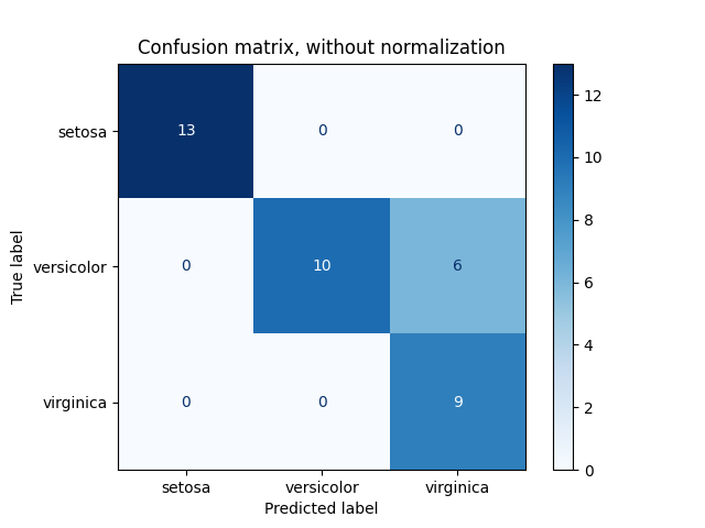
参数 normalize 允许报告比率而不是计数。混淆矩阵可以通过三种不同的方式进行归一化： 'pred' , 'true' ，而且 'all' 它将分别将计数除以每列、每行或整个矩阵的和。

>>> y_true = [0, 0, 0, 1, 1, 1, 1, 1]
>>> y_pred = [0, 1, 0, 1, 0, 1, 0, 1]
>>> confusion_matrix(y_true, y_pred, normalize='all')
array([[0.25 , 0.125],
       [0.25 , 0.375]])

对于二元问题，我们可以获得真阴性、假阳性、假阴性和真阳性的计数如下：

>>> y_true = [0, 0, 0, 1, 1, 1, 1, 1]
>>> y_pred = [0, 1, 0, 1, 0, 1, 0, 1]
>>> tn, fp, fn, tp = confusion_matrix(y_true, y_pred).ravel().tolist()
>>> tn, fp, fn, tp
(2, 1, 2, 3)

示例

• 看到 混淆矩阵 例如使用混淆矩阵来评估分类器输出质量。

• 看到 识别手写数字 使用混淆矩阵对手写数字进行分类的示例。

• 看到 使用稀疏特征对文本文档进行分类 使用混淆矩阵对文本文档进行分类的示例。

3.4.4.7. 分类报告

的 classification_report 函数构建一个显示主要分类指标的文本报告。下面是一个自定义的小例子 target_names 和推断的标签：：

>>> from sklearn.metrics import classification_report
>>> y_true = [0, 1, 2, 2, 0]
>>> y_pred = [0, 0, 2, 1, 0]
>>> target_names = ['class 0', 'class 1', 'class 2']
>>> print(classification_report(y_true, y_pred, target_names=target_names))
              precision    recall  f1-score   support

     class 0       0.67      1.00      0.80         2
     class 1       0.00      0.00      0.00         1
     class 2       1.00      0.50      0.67         2

    accuracy                           0.60         5
   macro avg       0.56      0.50      0.49         5
weighted avg       0.67      0.60      0.59         5

示例

• 看到 识别手写数字 用于手写数字的分类报告使用示例。

• 看到 具有交叉验证的网格搜索自定义改装策略 查看具有嵌套交叉验证的网格搜索的分类报告使用示例。

3.4.4.8. 海明损失

The hamming_loss computes the average Hamming loss or Hamming distance between two sets of samples.

如果 \(\hat{y}_{i,j}\) 是 \(j\) 给定样本的第-个标签 \(i\) , \(y_{i,j}\) 是相应的真值， \(n_\text{samples}\) 是样本数量和 \(n_\text{labels}\) 是标签的数量，然后是海明损失 \(L_{Hamming}\) 定义为：

\[L_{Hamming}(y, \hat{y}) = \frac{1}{n_\text{samples} * n_\text{labels}} \sum_{i=0}^{n_\text{samples}-1} \sum_{j=0}^{n_\text{labels} - 1} 1(\hat{y}_{i,j} \not= y_{i,j})\]

哪里 \(1(x)\) 是 indicator function .

在多类分类的情况下，上面的等式不成立。请参阅下面的注释以了解更多信息。:

>>> from sklearn.metrics import hamming_loss
>>> y_pred = [1, 2, 3, 4]
>>> y_true = [2, 2, 3, 4]
>>> hamming_loss(y_true, y_pred)
0.25

在具有二进制标签指示符的多标签情况下：：

>>> hamming_loss(np.array([[0, 1], [1, 1]]), np.zeros((2, 2)))
0.75

备注

在多类分类中，海明损失对应于 y_true 和 y_pred 类似于 零一损失 功能 然而，虽然0 - 1损失惩罚不严格匹配真集的预测集，但汉明损失惩罚单个标签。 因此，汉明损失的上限为0 - 1，总是在0和1之间，包括0和1;预测真标签的真子集或超集将给出介于0和1之间的汉明损失，不包括0和1。

3.4.4.9. 精确度、召回和F指标

直觉上， precision 分类器不将阴性样本标记为阳性的能力，以及 recall 是分类器找到所有阳性样本的能力。

The F-measure (\(F_\beta\) and \(F_1\) measures) can be interpreted as a weighted harmonic mean of the precision and recall. A \(F_\beta\) measure reaches its best value at 1 and its worst score at 0. With \(\beta = 1\), \(F_\beta\) and \(F_1\) are equivalent, and the recall and the precision are equally important.

的 precision_recall_curve 通过改变决策阈值，根据基本事实标签和分类器给出的分数计算精确召回曲线。

的 average_precision_score 函数计算 average precision (AP)来自预测分数。该值在0和1之间，越高越好。AP的定义是

\[\text{AP} = \sum_n（R_n-R_{n-1}）P_n\]

哪里 \(P_n\) 和 \(R_n\) 是第n个阈值处的准确率和召回率。对于随机预测，AP是阳性样本的分数。

引用 [Manning2008] 和 [Everingham2010] 提出了插入准确率-召回曲线的AP的替代变体。目前， average_precision_score 不实现任何内插变体。引用 [Davis2006] 和 [Flach2015] 描述为什么精确度-召回率曲线上的点的线性插值提供了对分类器性能的过于乐观的测量。当使用梯形规则计算曲线下的面积时，使用此线性插值， auc .

有几个功能可以让您分析精确度、召回率和F-测量分数：

average_precision_score(y_true, y_score, *)	根据预测分数计算平均精度（AP）。
f1_score(y_true, y_pred, *[, labels, ...])	计算F1评分，也称为平衡F评分或F测量。
fbeta_score(y_true, y_pred, *, beta[, ...])	计算F-beta评分。
precision_recall_curve(y_true[, y_score, ...])	Compute precision-recall pairs for different probability thresholds.
precision_recall_fscore_support(y_true, ...)	计算每个类的精确度、召回率、F-测度和支持度。
precision_score(y_true, y_pred, *[, labels, ...])	计算精度。
recall_score(y_true, y_pred, *[, labels, ...])	计算召回。

注意到 precision_recall_curve 函数仅限于二进制情况。的 average_precision_score 函数通过以One vs the rest（OvR）的方式计算每个类别分数并根据其平均值或不平均来支持多类别和多标签格式 average 参数值。

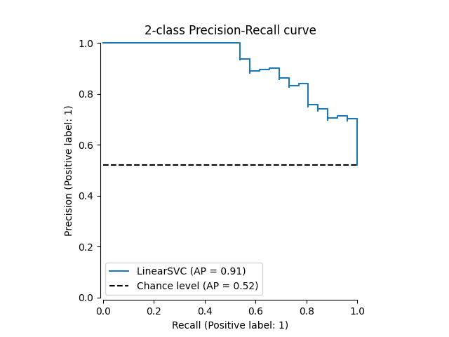
的 PrecisionRecallDisplay.from_estimator 和 PrecisionRecallDisplay.from_predictions 函数将绘制准确率-召回曲线如下。

示例

• 看到 具有交叉验证的网格搜索自定义改装策略 的示例 precision_score 和 recall_score 用于使用网格搜索和嵌套交叉验证来估计参数。

• 看到 pr曲线 的示例 precision_recall_curve 用于评估分类器输出质量。

引用

[Manning2008]

C.D.曼宁，P. Raghavan，H.许策， Introduction to Information Retrieval ，2008年。

[Everingham2010]

M.埃弗灵厄姆湖范古尔，CKI威廉姆斯，J. Winn，A.齐瑟曼， The Pascal Visual Object Classes (VOC) Challenge ，IJCV 2010。

[Davis2006]

J. Davis, M. Goadrich, The Relationship Between Precision-Recall and ROC Curves, ICML 2006.

[Flach2015]

P.A. Flach，M.库尔， Precision-Recall-Gain Curves: PR Analysis Done Right ，NIPS 2015。

3.4.4.9.1. 二元分类

在二元分类任务中，术语“积极”和“消极”是指分类器的预测，术语“真”和“假”是指该预测是否对应于外部判断（有时称为“观察”）。鉴于这些定义，我们可以制定下表：

	实际班级（观察）
预测班级（期望）	tp（真阳性）正确结果	FP（假阳性）意外结果
	fn（假阴性）缺失结果	tn (true negative) Correct absence of result

在这种情况下，我们可以定义精确度和召回率的概念：

\[\text{precision} = \frac{\text{tp}}{\text{tp} + \text{fp}},\]

\[\text{recall} = \frac{\text{tp}}{\text{tp} + \text{fn}},\]

（有时回忆也被称为“敏感性”）

F-测量是精确度和召回率的加权调和平均值，精确度对平均值的贡献由某个参数加权 \(\beta\) :

\[F_\beta = (1 + \beta^2) \frac{\text{precision} \times \text{recall}}{\beta^2 \text{precision} + \text{recall}}\]

为了避免在精度和召回率为零时被零除，Scikit-Learn使用这个其他等效公式计算F测量：

\[F_\beta = \frac{(1 + \beta^2) \text{tp}}{(1 + \beta^2) \text{tp} + \text{fp} + \beta^2 \text{fn}}\]

请注意，当没有真阳性、假阳性或假阴性时，此公式仍然未定义。默认情况下，一组排他性真负的F-1计算为0，但可以使用 zero_division 参数.下面是一些二进制分类的小例子：

>>> from sklearn import metrics
>>> y_pred = [0, 1, 0, 0]
>>> y_true = [0, 1, 0, 1]
>>> metrics.precision_score(y_true, y_pred)
1.0
>>> metrics.recall_score(y_true, y_pred)
0.5
>>> metrics.f1_score(y_true, y_pred)
0.66
>>> metrics.fbeta_score(y_true, y_pred, beta=0.5)
0.83
>>> metrics.fbeta_score(y_true, y_pred, beta=1)
0.66
>>> metrics.fbeta_score(y_true, y_pred, beta=2)
0.55
>>> metrics.precision_recall_fscore_support(y_true, y_pred, beta=0.5)
(array([0.66, 1.        ]), array([1. , 0.5]), array([0.71, 0.83]), array([2, 2]))


>>> import numpy as np
>>> from sklearn.metrics import precision_recall_curve
>>> from sklearn.metrics import average_precision_score
>>> y_true = np.array([0, 0, 1, 1])
>>> y_scores = np.array([0.1, 0.4, 0.35, 0.8])
>>> precision, recall, threshold = precision_recall_curve(y_true, y_scores)
>>> precision
array([0.5       , 0.66, 0.5       , 1.        , 1.        ])
>>> recall
array([1. , 1. , 0.5, 0.5, 0. ])
>>> threshold
array([0.1 , 0.35, 0.4 , 0.8 ])
>>> average_precision_score(y_true, y_scores)
0.83

3.4.4.9.2. 多类别和多标签分类

在多类别和多标签分类任务中，精确度、召回率和F-测量的概念可以独立应用于每个标签。有几种方法可以组合跨标签的结果，具体由 average 论点 average_precision_score , f1_score , fbeta_score , precision_recall_fscore_support , precision_score 和 recall_score 功能，如所述 above .

求平均时请注意以下行为：

• 如果包括所有标签，那么多类设置中的“微”平均将产生精确度、召回率和 \(F\) 这些都与准确性相同。

• “加权”平均可能会产生不在精确度和召回率之间的F分数。

• F测量的“宏”平均计算为每个标签/类别F测量的算术平均值，而不是算术精度和召回平均值的调和平均值。这两种计算都可以在文献中看到，但不等效，请参阅 [OB2019] 有关详细信息

为了使其更加明确，请考虑以下符号：

• \(y\) 该组 true \((sample, label)\) 对

• \(\hat{y}\) 该组 predicted \((sample, label)\) 对

• \(L\) 标签的集合

• \(S\) 该样本集合

• \(y_s\) the subset of \(y\) with sample \(s\), i.e. \(y_s := \left\{(s', l) \in y | s' = s\right\}\)

• \(y_l\) 的子集 \(y\) with label \(l\)

• 类似地， \(\hat{y}_s\) 和 \(\hat{y}_l\) 是的子集 \(\hat{y}\)

• \(P(A, B) := \frac{\left| A \cap B \right|}{\left|B\right|}\) for some sets \(A\) and \(B\)

• \(R(A, B) := \frac{\left| A \cap B \right|}{\left|A\right|}\) (Conventions vary on handling \(A = \emptyset\); this implementation uses \(R(A, B):=0\), and similar for \(P\).)

• \(F_\beta(A, B) := \left(1 + \beta^2\right) \frac{P(A, B) \times R(A, B)}{\beta^2 P(A, B) + R(A, B)}\)

然后指标定义为：

average	精度	召回	F_beta
"micro"	\(P(y, \hat{y})\)	\(R(y, \hat{y})\)	\(F_\beta(y, \hat{y})\)
"samples"	\(\frac{1}{\left|S\right|} \sum_{s \in S} P(y_s, \hat{y}_s)\)	\(\frac{1}{\left|S\right|} \sum_{s \in S} R(y_s, \hat{y}_s)\)	\(\frac{1}{\left|S\right|} \sum_{s \in S} F_\beta(y_s, \hat{y}_s)\)
"macro"	\(\frac{1}{\left|L\right|} \sum_{l \in L} P(y_l, \hat{y}_l)\)	\(\frac{1}{\left|L\right|} \sum_{l \in L} R(y_l, \hat{y}_l)\)	\(\frac{1}{\left|L\right|} \sum_{l \in L} F_\beta(y_l, \hat{y}_l)\)
"weighted"	\(\frac{1}{\sum_{l \in L} \left|y_l\right|} \sum_{l \in L} \left|y_l\right| P(y_l, \hat{y}_l)\)	\(\frac{1}{\sum_{l \in L} \left|y_l\right|} \sum_{l \in L} \left|y_l\right| R(y_l, \hat{y}_l)\)	\(\frac{1}{\sum_{l \in L} \left|y_l\right|} \sum_{l \in L} \left|y_l\right| F_\beta(y_l, \hat{y}_l)\)
None	\(\langle P(y_l, \hat{y}_l) | l \in L \rangle\)	\(\langle R(y_l, \hat{y}_l) | l \in L \rangle\)	\(\langle F_\beta(y_l, \hat{y}_l) | l \in L \rangle\)

>>> from sklearn import metrics
>>> y_true = [0, 1, 2, 0, 1, 2]
>>> y_pred = [0, 2, 1, 0, 0, 1]
>>> metrics.precision_score(y_true, y_pred, average='macro')
0.22
>>> metrics.recall_score(y_true, y_pred, average='micro')
0.33
>>> metrics.f1_score(y_true, y_pred, average='weighted')
0.267
>>> metrics.fbeta_score(y_true, y_pred, average='macro', beta=0.5)
0.238
>>> metrics.precision_recall_fscore_support(y_true, y_pred, beta=0.5, average=None)
(array([0.667, 0., 0.]), array([1., 0., 0.]), array([0.714, 0., 0.]), array([2, 2, 2]))

对于具有“负类”的多类分类，可以排除一些标签：

>>> metrics.recall_score(y_true, y_pred, labels=[1, 2], average='micro')
... # excluding 0, no labels were correctly recalled
0.0

同样，数据样本中不存在的标签可以在宏观平均中考虑。

>>> metrics.precision_score(y_true, y_pred, labels=[0, 1, 2, 3], average='macro')
0.166

引用

[OB2019]

Opitz, J., & Burst, S. (2019). "Macro f1 and macro f1."

3.4.4.10. 贾卡德相似系数得分

的 jaccard_score 函数计算的平均值 Jaccard similarity coefficients ，也称为Jaccard索引，位于标签集对之间。

The Jaccard similarity coefficient with a ground truth label set \(y\) and predicted label set \(\hat{y}\), is defined as

\[J(y, \hat{y}) = \frac{|y \cap \hat{y}|}{|y \cup \hat{y}|}.\]

的 jaccard_score （喜欢 precision_recall_fscore_support ）本机适用于二元目标。通过按集合计算，它可以通过使用扩展来应用于多标签和多类 average （见 above ).

在二进制情况下：：

>>> import numpy as np
>>> from sklearn.metrics import jaccard_score
>>> y_true = np.array([[0, 1, 1],
...                    [1, 1, 0]])
>>> y_pred = np.array([[1, 1, 1],
...                    [1, 0, 0]])
>>> jaccard_score(y_true[0], y_pred[0])
0.6666

在2D比较情况下（例如图像相似性）：

>>> jaccard_score(y_true, y_pred, average="micro")
0.6

在具有二进制标签指示符的多标签情况下：：

>>> jaccard_score(y_true, y_pred, average='samples')
0.5833
>>> jaccard_score(y_true, y_pred, average='macro')
0.6666
>>> jaccard_score(y_true, y_pred, average=None)
array([0.5, 0.5, 1. ])

多类问题被二进制化，并像相应的多标签问题一样处理：：

>>> y_pred = [0, 2, 1, 2]
>>> y_true = [0, 1, 2, 2]
>>> jaccard_score(y_true, y_pred, average=None)
array([1. , 0. , 0.33])
>>> jaccard_score(y_true, y_pred, average='macro')
0.44
>>> jaccard_score(y_true, y_pred, average='micro')
0.33

3.4.4.11. 铰链损耗

的 hinge_loss 函数使用计算模型和数据之间的平均距离 hinge loss ，一个仅考虑预测误差的单边指标。（铰链损失用于最大裕度分类器，例如支持向量机。）

If the true label \(y_i\) of a binary classification task is encoded as \(y_i=\left\{-1, +1\right\}\) for every sample \(i\); and \(w_i\) is the corresponding predicted decision (an array of shape (n_samples,) as output by the decision_function method), then the hinge loss is defined as:

\[L_\text{Hinge}(y, w) = \frac{1}{n_\text{samples}} \sum_{i=0}^{n_\text{samples}-1} \max\left\{1 - w_i y_i, 0\right\}\]

如果有两个以上的标签， hinge_loss 由于Crammer & Singer，使用了多类变体。 Here 是描述它的论文。

In this case the predicted decision is an array of shape (n_samples, n_labels). If \(w_{i, y_i}\) is the predicted decision for the true label \(y_i\) of the \(i\)-th sample; and \(\hat{w}_{i, y_i} = \max\left\{w_{i, y_j}~|~y_j \ne y_i \right\}\) is the maximum of the predicted decisions for all the other labels, then the multi-class hinge loss is defined by:

\[L_\text{Hinge}(y, w) = \frac{1}{n_\text{samples}} \sum_{i=0}^{n_\text{samples}-1} \max\left\{1 + \hat{w}_{i, y_i} - w_{i, y_i}, 0\right\}\]

这是一个小示例，演示了 hinge_loss 二进制类问题中具有svm分类器的函数：：

>>> from sklearn import svm
>>> from sklearn.metrics import hinge_loss
>>> X = [[0], [1]]
>>> y = [-1, 1]
>>> est = svm.LinearSVC(random_state=0)
>>> est.fit(X, y)
LinearSVC(random_state=0)
>>> pred_decision = est.decision_function([[-2], [3], [0.5]])
>>> pred_decision
array([-2.18,  2.36,  0.09])
>>> hinge_loss([-1, 1, 1], pred_decision)
0.3

以下是一个示例演示 hinge_loss 多类问题中具有svm分类器的函数：：

>>> X = np.array([[0], [1], [2], [3]])
>>> Y = np.array([0, 1, 2, 3])
>>> labels = np.array([0, 1, 2, 3])
>>> est = svm.LinearSVC()
>>> est.fit(X, Y)
LinearSVC()
>>> pred_decision = est.decision_function([[-1], [2], [3]])
>>> y_true = [0, 2, 3]
>>> hinge_loss(y_true, pred_decision, labels=labels)
0.56

3.4.4.12. 对数损失

Log loss, also called logistic regression loss or cross-entropy loss, is defined on probability estimates. It is commonly used in (multinomial) logistic regression and neural networks, as well as in some variants of expectation-maximization, and can be used to evaluate the probability outputs (predict_proba) of a classifier instead of its discrete predictions.

For binary classification with a true label \(y \in \{0,1\}\) and a probability estimate \(\hat{p} \approx \operatorname{Pr}(y = 1)\), the log loss per sample is the negative log-likelihood of the classifier given the true label:

\[L_{\log}(y, \hat{p}) = -\log \operatorname{Pr}(y|\hat{p}) = -(y \log (\hat{p}) + (1 - y) \log (1 - \hat{p}))\]

This extends to the multiclass case as follows. Let the true labels for a set of samples be encoded as a 1-of-K binary indicator matrix \(Y\), i.e., \(y_{i,k} = 1\) if sample \(i\) has label \(k\) taken from a set of \(K\) labels. Let \(\hat{P}\) be a matrix of probability estimates, with elements \(\hat{p}_{i,k} \approx \operatorname{Pr}(y_{i,k} = 1)\). Then the log loss of the whole set is

\[L_{\log}(Y, \hat{P}) = -\log \operatorname{Pr}(Y|\hat{P}) = - \frac{1}{N} \sum_{i=0}^{N-1} \sum_{k=0}^{K-1} y_{i,k} \log \hat{p}_{i,k}\]

To see how this generalizes the binary log loss given above, note that in the binary case, \(\hat{p}_{i,0} = 1 - \hat{p}_{i,1}\) and \(y_{i,0} = 1 - y_{i,1}\), so expanding the inner sum over \(y_{i,k} \in \{0,1\}\) gives the binary log loss.

的 log_loss 给定地面真值标签列表和概率矩阵（由估计器返回），函数计算日志损失 predict_proba 法

>>> from sklearn.metrics import log_loss
>>> y_true = [0, 0, 1, 1]
>>> y_pred = [[.9, .1], [.8, .2], [.3, .7], [.01, .99]]
>>> log_loss(y_true, y_pred)
0.1738

第一 [.9, .1] 在 y_pred 表示第一个样本具有标记0的可能性为90%。 对数损失是非负的。

3.4.4.13. 马修斯相关系数

的 matthews_corrcoef 函数计算 Matthew's correlation coefficient (MCC) 对于二进制类。 引用维基百科：

“马修斯相关系数用于机器学习中，作为二元（两类）分类质量的衡量标准。它考虑了真阳性、假阳性和阴性，通常被认为是一种平衡的衡量标准，即使类别的规模差异很大，也可以使用。MCC本质上是-1和+1之间的相关系数值。系数+1代表完美预测，0代表平均随机预测，-1代表逆预测。该统计数据也称为ph系数。"

在二进制（两类）情况下， \(tp\) , \(tn\) , \(fp\) 和 \(fn\) 分别是真阳性、真阴性、假阳性和假阴性的数量，MCC定义为

\[MCC = \frac{tp \times tn - fp \times fn}{\sqrt{(tp + fp)(tp + fn)(tn + fp)(tn + fn)}}.\]

在多类情况下，马修斯相关系数可以是 defined 用一个 confusion_matrix \(C\) 为 \(K\) 班 为了简化定义，请考虑以下中间变量：

• \(t_k=\sum_{i}^{K} C_{ik}\) 上课次数 \(k\) 确实发生了，

• \(p_k=\sum_{i}^{K} C_{ki}\) 上课次数 \(k\) 被预测，

• \(c=\sum_{k}^{K} C_{kk}\) 正确预测的样本总数，

• \(s=\sum_{i}^{K} \sum_{j}^{K} C_{ij}\) 样本总数。

那么多类MCC定义为：

\[MCC = \frac{ c \times s - \sum_{k}^{K} p_k \times t_k }{\sqrt{ (s^2 - \sum_{k}^{K} p_k^2) \times (s^2 - \sum_{k}^{K} t_k^2) }}\]

当有两个以上的标签时，MCC的值将不再介于-1和+1之间。相反，最小值将介于-1和0之间，具体取决于地面真值标签的数量和分布。最大值始终为+1。更多信息请参见 [WikipediaMCC2021].

这是一个小示例，说明 matthews_corrcoef 功能：

>>> from sklearn.metrics import matthews_corrcoef
>>> y_true = [+1, +1, +1, -1]
>>> y_pred = [+1, -1, +1, +1]
>>> matthews_corrcoef(y_true, y_pred)
-0.33

引用

[WikipediaMCC2021]

维基百科贡献者。Phi系数。维基百科，自由百科全书。2021年4月21日，英国中部时间12：21。可访问：https://en.wikipedia.org/wiki/Phi_coefficient访问于2021年4月21日。

3.4.4.14. 多标签混淆矩阵

的 multilabel_confusion_matrix 函数计算逐类（默认）或逐样本（samplewise=True）多标签混淆矩阵以评估分类的准确性。MultilLabel_conflict_matrix还将多类数据视为多标签，因为这是一种通常应用于使用二进制分类指标（例如精度、召回率等）评估多类问题的转换。

计算逐类多标签混淆矩阵时 \(C\) ，类的真阴性计数 \(i\) 是 \(C_{i,0,0}\) ，假阴性是 \(C_{i,1,0}\) ，真正的积极因素是 \(C_{i,1,1}\) 假阳性是 \(C_{i,0,1}\) .

以下是一个示例演示 multilabel_confusion_matrix 函数 multilabel indicator matrix 输入：：

>>> import numpy as np
>>> from sklearn.metrics import multilabel_confusion_matrix
>>> y_true = np.array([[1, 0, 1],
...                    [0, 1, 0]])
>>> y_pred = np.array([[1, 0, 0],
...                    [0, 1, 1]])
>>> multilabel_confusion_matrix(y_true, y_pred)
array([[[1, 0],
        [0, 1]],

       [[1, 0],
        [0, 1]],

       [[0, 1],
        [1, 0]]])

或者可以为每个样本的标签构建混淆矩阵：

>>> multilabel_confusion_matrix(y_true, y_pred, samplewise=True)
array([[[1, 0],
        [1, 1]],

       [[1, 1],
        [0, 1]]])

以下是一个示例演示 multilabel_confusion_matrix 函数 multiclass 输入：：

>>> y_true = ["cat", "ant", "cat", "cat", "ant", "bird"]
>>> y_pred = ["ant", "ant", "cat", "cat", "ant", "cat"]
>>> multilabel_confusion_matrix(y_true, y_pred,
...                             labels=["ant", "bird", "cat"])
array([[[3, 1],
        [0, 2]],

       [[5, 0],
        [1, 0]],

       [[2, 1],
        [1, 2]]])

以下是一些示例演示 multilabel_confusion_matrix 功能用于计算具有多标签指标矩阵输入的问题中每个类别的召回率（或敏感性）、特异性、脱落率和遗漏率。

计算 recall (also称为真阳性率或灵敏度）为每个类别：：

>>> y_true = np.array([[0, 0, 1],
...                    [0, 1, 0],
...                    [1, 1, 0]])
>>> y_pred = np.array([[0, 1, 0],
...                    [0, 0, 1],
...                    [1, 1, 0]])
>>> mcm = multilabel_confusion_matrix(y_true, y_pred)
>>> tn = mcm[:, 0, 0]
>>> tp = mcm[:, 1, 1]
>>> fn = mcm[:, 1, 0]
>>> fp = mcm[:, 0, 1]
>>> tp / (tp + fn)
array([1. , 0.5, 0. ])

计算 specificity (also称为真负率）为每个类别：：

>>> tn / (tn + fp)
array([1. , 0. , 0.5])

计算 fall out (also称为假阳性率）为每个类别：：

>>> fp / (fp + tn)
array([0. , 1. , 0.5])

计算 miss rate (also称为假阴性率）为每个类别：：

>>> fn / (fn + tp)
array([0. , 0.5, 1. ])

3.4.4.15. 接收器工作特性（ROC）

功能 roc_curve 来计算 receiver operating characteristic curve, or ROC curve .引用维基百科：

“接收器工作特征（ROC），或简称为ROC曲线，是一个图形图，说明了二元分类器系统在区分阈值变化时的性能。它是通过绘制各种阈值设置下阳性中的真阳性比例（TPR =真阳性率）与阴性中的假阳性比例（FPR =假阳性率）绘制的。TPA也称为敏感性，FPR是一减去特异性或真阴性率。"

此函数需要真实的二进制值和目标分数，目标分数可以是正类的概率估计值、置信度值或二进制决策。下面是一个小示例，说明如何使用 roc_curve 功能：：

>>> import numpy as np
>>> from sklearn.metrics import roc_curve
>>> y = np.array([1, 1, 2, 2])
>>> scores = np.array([0.1, 0.4, 0.35, 0.8])
>>> fpr, tpr, thresholds = roc_curve(y, scores, pos_label=2)
>>> fpr
array([0. , 0. , 0.5, 0.5, 1. ])
>>> tpr
array([0. , 0.5, 0.5, 1. , 1. ])
>>> thresholds
array([ inf, 0.8 , 0.4 , 0.35, 0.1 ])

与子集准确性、汉明损失或F1得分等指标相比，ROC不需要为每个标签优化阈值。

的 roc_auc_score 用ROC-AUROC或AUROC表示的函数计算ROC曲线下面积。通过这样做，曲线信息被总结为一个数字。

下图显示了旨在将Virginica花与其他物种区分开来的分类器的ROC曲线和ROC-UC评分。 虹膜植物数据集 :

有关更多信息，请参阅 Wikipedia article on AUC .

3.4.4.15.1. 二进制情况

在 binary case ，您可以使用 classifier.predict_proba() 方法，或由 classifier.decision_function() 法在提供概率估计的情况下，应提供具有“更大标签”的类别的概率。“更大的标签”对应于 classifier.classes_[1] 并且因此 classifier.predict_proba(X)[:, 1] .因此 y_score 参数的大小为（n_samples，）。

>>> from sklearn.datasets import load_breast_cancer
>>> from sklearn.linear_model import LogisticRegression
>>> from sklearn.metrics import roc_auc_score
>>> X, y = load_breast_cancer(return_X_y=True)
>>> clf = LogisticRegression().fit(X, y)
>>> clf.classes_
array([0, 1])

我们可以使用相应的概率估计， clf.classes_[1] .

>>> y_score = clf.predict_proba(X)[:, 1]
>>> roc_auc_score(y, y_score)
0.99

否则，我们可以使用非阈值决策值

>>> roc_auc_score(y, clf.decision_function(X))
0.99

3.4.4.15.2. 多类案例

的 roc_auc_score 功能也可以用于 multi-class classification .目前支持两种求平均策略：一对一算法计算成对的ROC AUC分数的平均值，而一对休息算法计算每个类别与所有其他类别的ROC AUC分数的平均值。在这两种情况下，预测的标签都以值从0到 n_classes ，并且分数对应于样本属于特定类别的概率估计。OvO和OvR算法支持统一加权 (average='macro' ）和按患病率 (average='weighted' ).

一对一算法

计算所有可能的类别成对组合的平均曲线下面积。 [HT2001] 定义均匀加权的多类AUT指标：

\[\frac{1}{c(c-1)}\sum_{j=1}^{c}\sum_{k > j}^c (\text{AUC}(j | k) + \text{AUC}(k | j))\]

where \(c\) is the number of classes and \(\text{AUC}(j | k)\) is the AUC with class \(j\) as the positive class and class \(k\) as the negative class. In general, \(\text{AUC}(j | k) \neq \text{AUC}(k | j))\) in the multiclass case. This algorithm is used by setting the keyword argument multiclass to 'ovo' and average to 'macro'.

的 [HT2001] 多类AUT指标可以扩展为通过患病率加权：

\[\frac{1}{c(c-1)}\sum_{j=1}^{c}\sum_{k > j}^c p(j \cup k)( \text{AUC}(j | k) + \text{AUC}(k | j))\]

哪里 \(c\) 是类的数量。通过设置关键字参数来使用该算法 multiclass 到 'ovo' 和 average 到 'weighted' .的 'weighted' 选项返回中所述的流行率加权平均值 [FC2009].

One-vs-rest Algorithm

计算每个类别与其他类别的UC [PD2000]. 该算法在功能上与多标签情况相同。要启用此算法，请设置关键字参数 multiclass 到 'ovr' .可另外实施的 'macro' [F2006] 和 'weighted' [F2001] 平均，OvR支持 'micro' 平均。

在无法容忍高假阳性率的应用中，参数 max_fpr 的 roc_auc_score 可用于总结给定限制的ROC曲线。

下图显示了微平均ROC曲线及其相应的ROC-AUC评分，用于区分不同物种的分类器。 虹膜植物数据集 :

3.4.4.15.3. 多标签案例

在 multi-label classification ， roc_auc_score 通过对标签进行平均来扩展函数为 above .在这种情况下，您应该提供 y_score 形状 (n_samples, n_classes) .因此，当使用概率估计时，需要为每个输出选择具有更大标签的类的概率。

>>> from sklearn.datasets import make_multilabel_classification
>>> from sklearn.multioutput import MultiOutputClassifier
>>> X, y = make_multilabel_classification(random_state=0)
>>> inner_clf = LogisticRegression(random_state=0)
>>> clf = MultiOutputClassifier(inner_clf).fit(X, y)
>>> y_score = np.transpose([y_pred[:, 1] for y_pred in clf.predict_proba(X)])
>>> roc_auc_score(y, y_score, average=None)
array([0.828, 0.851, 0.94, 0.87, 0.95])

并且决策值不需要这样的处理。

>>> from sklearn.linear_model import RidgeClassifierCV
>>> clf = RidgeClassifierCV().fit(X, y)
>>> y_score = clf.decision_function(X)
>>> roc_auc_score(y, y_score, average=None)
array([0.82, 0.85, 0.93, 0.87, 0.94])

示例

• 看到 sphx_glr_auto_examples_model_selection_plot_roc.py 使用ROC评估分类器输出质量的示例。

• 看到 具有交叉验证的接收器工作特性（ROC） 对于使用ROC来评估分类器输出质量的示例，使用交叉验证。

• See 物种分布建模 for an example of using ROC to model species distribution.

引用

[HT2001] (1,2)

DJ汉德和RJ蒂尔（2001）。 A simple generalisation of the area under the ROC curve for multiple class classification problems. 机器学习，45（2），pp。171-186.

[FC2009]

Ferri，Cèsar & Hernandez-Orallo，Jose & Modroiu，R.（2009）。 An Experimental Comparison of Performance Measures for Classification. 模式识别字母。30. 27-38.

[PD2000]

教务长，F.，Domingos，P.（2000年）。 Well-trained PETs: Improving probability estimation trees （第6.2节），CeGER工作文件#IS-00-04，纽约大学斯特恩商学院。

[F2006]

福塞特，T.，2006. An introduction to ROC analysis. 模式识别信件，27（8），pp。861-874.

[F2001]

福塞特，T.，2001. Using rule sets to maximize ROC performance 数据挖掘，2001年。IEEE国际会议文集，pp。131-138.

3.4.4.16. 检测错误权衡（DET）

功能 det_curve 计算检测误差权衡曲线（DET）曲线 [WikipediaDET2017]. 引用维基百科：

“检测错误权衡（DET）图是二进制分类系统错误率的图形图，绘制了错误拒绝率与错误接受率。x轴和y轴通过其标准正态偏差（或仅通过对数变换）进行非线性缩放，从而产生比ROC曲线更线性的权衡曲线，并使用大部分图像区域来突出关键操作区域中重要性的差异。"

DET曲线是接受者工作特性（ROC）曲线的变体，其中假阴性率绘制在y轴上，而不是真阳性率。DET曲线通常通过以下方式绘制成正态偏差标度 \(\phi^{-1}\) （与 \(\phi\) 是累积分布函数）。由此产生的性能曲线显式地可视化了给定分类算法的错误类型的权衡。看到 [Martin1997] 以获取例子和进一步的动机。

此图比较了同一分类任务下两个示例分类器的ROC和DET曲线：

性能

• 如果检测分数正态（或接近正态）分布，DET曲线在正态偏差量表中形成线性曲线。它是由 [Navratil2007] 相反的情况不一定成立，甚至更一般的分布也能够产生线性DET曲线。

• 正常偏离比例变换将点展开，从而占据相对较大的地块空间。因此，具有相似分类性能的曲线在DET图上可能更容易区分。

• 假阴性率与真阳性率“相反”，DET曲线的完美点是起点（与ROC曲线的左上角相反）。

应用以及局限性方面

DET曲线易于直观阅读，因此允许对分类器的性能进行快速视觉评估。此外，可以参考DET曲线进行阈值分析和操作点选择。如果需要比较错误类型，这尤其有帮助。

另一方面，DET曲线不会将其指标作为单个数字提供。因此，对于自动评估或与其他分类任务的比较，ROC曲线下的推导面积等指标可能更适合。

示例

• 看到 sphx_glr_auto_examples_model_selection_plot_det.py 接收器工作特性（ROC）曲线和检测误差权衡（DET）曲线之间的示例比较。

引用

[WikipediaDET2017]

维基百科贡献者。检测错误权衡。维基百科，自由百科全书。协调世界时2017年9月4日23：33。可访问：https://en.wikipedia.org/w/index.php? title=Detection_error_tradeoff < oldid=798982054。访问于2018年2月19日。

[Martin1997]

A.马丁，G。多丁顿，T.卡姆，M.奥尔多夫斯基和M.普日博茨基， The DET Curve in Assessment of Detection Task Performance ，NIH 1997年。

[Navratil2007]

J. Navratil and D. Klusacek, "On Linear DETs", 2007 IEEE International Conference on Acoustics, Speech and Signal Processing - ICASSP '07, Honolulu, HI, 2007, pp. IV-229-IV-232.

3.4.4.17. 零一损失

的 zero_one_loss 函数计算0-1分类损失的总和或平均值 (\(L_{0-1}\) ）结束 \(n_{\text{samples}}\) .默认情况下，该函数会对样本进行规格化。要得到的总和 \(L_{0-1}\) ，设置 normalize 到 False .

在多标签分类中， zero_one_loss 如果子集的标签严格匹配预测，则将其评分为一，如果存在任何错误，则将其评分为零。 默认情况下，该函数返回不完全预测的子集的百分比。 要获取此类子集的计数，请设置 normalize 到 False .

如果 \(\hat{y}_i\) 是 \(i\) -th样本， \(y_i\) 是相应的真值，那么0-1损失 \(L_{0-1}\) 定义为：

\[L_{0-1}(y, \hat{y}) = \frac{1}{n_\text{samples}} \sum_{i=0}^{n_\text{samples}-1} 1(\hat{y}_i \not= y_i)\]

哪里 \(1(x)\) 是 indicator function .零零一损失也可以计算为 \(\text{zero-one loss} = 1 - \text{accuracy}\) .

>>> from sklearn.metrics import zero_one_loss
>>> y_pred = [1, 2, 3, 4]
>>> y_true = [2, 2, 3, 4]
>>> zero_one_loss(y_true, y_pred)
0.25
>>> zero_one_loss(y_true, y_pred, normalize=False)
1.0

在具有二进制标签指示符的多标签情况下，其中第一个标签集 [0,1] 有一个错误：：

>>> zero_one_loss(np.array([[0, 1], [1, 1]]), np.ones((2, 2)))
0.5

>>> zero_one_loss(np.array([[0, 1], [1, 1]]), np.ones((2, 2)),  normalize=False)
1.0

示例

• 看到 sphx_glr_auto_examples_feature_selection_plot_rfe_with_cross_validation.py 使用零一一损失来执行通过交叉验证的循环特征消除的示例。

3.4.4.18. Brier score loss

的 brier_score_loss 函数计算 Brier score 用于二进制和多类概率预测，相当于均方误差。引用维基百科：

"The Brier score is a strictly proper scoring rule that measures the accuracy of probabilistic predictions. [...] [It] is applicable to tasks in which predictions must assign probabilities to a set of mutually exclusive discrete outcomes or classes."

Let the true labels for a set of \(N\) data points be encoded as a 1-of-K binary indicator matrix \(Y\), i.e., \(y_{i,k} = 1\) if sample \(i\) has label \(k\) taken from a set of \(K\) labels. Let \(\hat{P}\) be a matrix of probability estimates with elements \(\hat{p}_{i,k} \approx \operatorname{Pr}(y_{i,k} = 1)\). Following the original definition by [Brier1950], the Brier score is given by:

\[BS(Y, \hat{P}) = \frac{1}{N}\sum_{i=0}^{N-1}\sum_{k=0}^{K-1}(y_{i,k} - \hat{p}_{i,k})^{2}\]

布里尔得分在于中场休息 \([0, 2]\) 并且该值越低，概率估计越好（均方差越小）。实际上，Brier评分是一个严格的评分规则，这意味着只有当估计的概率等于真实概率时，它才能获得最佳评分。

Note that in the binary case, the Brier score is usually divided by two and ranges between \([0,1]\). For binary targets \(y_i \in {0, 1}\) and probability estimates \(\hat{p}_i \approx \operatorname{Pr}(y_i = 1)\) for the positive class, the Brier score is then equal to:

\[BS(y, \hat{p}) = \frac{1}{N} \sum_{i=0}^{N - 1}(y_i - \hat{p}_i)^2\]

的 brier_score_loss 函数计算给定地面真相标签和预测概率（由估计器返回）的Brier分数 predict_proba 法的 scale_by_half 参数控制遵循上述两个定义中的哪一个。

>>> import numpy as np
>>> from sklearn.metrics import brier_score_loss
>>> y_true = np.array([0, 1, 1, 0])
>>> y_true_categorical = np.array(["spam", "ham", "ham", "spam"])
>>> y_prob = np.array([0.1, 0.9, 0.8, 0.4])
>>> brier_score_loss(y_true, y_prob)
0.055
>>> brier_score_loss(y_true, 1 - y_prob, pos_label=0)
0.055
>>> brier_score_loss(y_true_categorical, y_prob, pos_label="ham")
0.055
>>> brier_score_loss(
...    ["eggs", "ham", "spam"],
...    [[0.8, 0.1, 0.1], [0.2, 0.7, 0.1], [0.2, 0.2, 0.6]],
...    labels=["eggs", "ham", "spam"],
... )
0.146

Brier评分可用于评估分类器的校准程度。然而，较低的Brier评分损失并不总是意味着更好的校准。这是因为，通过与均方误差的偏差方差分解类比，Brier得分损失可以分解为校准损失和细化损失的和 [Bella2012]. 校准损失定义为从ROC段的斜坡得出的经验概率的均方偏差。细化损失可以定义为通过最佳成本曲线下的面积衡量的预期最佳损失。细化损失可以独立于校准损失而变化，因此较低的Brier评分损失并不一定意味着校准的模型更好。“只有当细化损失保持不变时，较低的Brier评分损失总是意味着更好的校准” [Bella2012], [Flach2008].

示例

• 看到 分类器的概率校准 使用Brier评分损失来执行分类器的概率校准的示例。

引用

[Brier1950]

G.布里尔， Verification of forecasts expressed in terms of probability 、每月天气回顾78.1（1950）

[Bella2012] (1,2)

贝拉、费里、埃尔南德斯-奥拉洛和拉米雷斯-金塔纳 "Calibration of Machine Learning Models" 在M.科斯罗普尔。“机器学习：概念、方法论、工具和应用。”宾夕法尼亚州好时：信息科学参考（2012年）。

[Flach2008]

Flach、Peter和Edson Matsubara。 "On classification, ranking, and probability estimation." 达格斯图尔研讨会会议记录。Schloss Dagstuhl-Leibniz-Zentrum für Informatik（2008）。

3.4.4.19. 类似然比

的 class_likelihood_ratios 函数计算 positive and negative likelihood ratios \(LR_\pm\) 对于二元类，可以解释为测试后与测试前的比值，如下所述。因此，这个度量是不变的w.r.t.类别患病率（阳性类别中的样本数除以样本总数），以及 can be extrapolated between populations regardless of any possible class imbalance.

的 \(LR_\pm\) 因此，指标在可用于学习和评估分类器的数据是具有近乎平衡类别的研究人群（例如病例对照研究）的环境中非常有用，而目标应用程序（即一般人群）的流行率非常低。

阳性似然比 \(LR_+\) 是分类器正确预测样本属于正类的概率除以预测属于负类的样本的正类的概率：

\[LR_+ = \fRAC{\text{PR}（P+| T+）}{\text{PR}（P+| T-）}。\]

这里的符号是指预测的 (\(P\) ）或真的 (\(T\) ）标签和标志 \(+\) 和 \(-\) 分别指正类和负类，例如 \(P+\) 代表“预测阳性”。

类似地，负似然比 \(LR_-\) 是正类样本被分类为属于负类的概率除以负类样本被正确分类的概率：

\[LR_- = \frac{\text{PR}(P-|T+)}{\text{PR}(P-|T-)}.\]

对于chance之上的分类器 \(LR_+\) 高于1 higher is better 而 \(LR_-\) 范围从0到1， lower is better .值 \(LR_\pm\approx 1\) 对应于机会水平。

请注意，例如，概率与计数不同 \(\operatorname{PR}(P+|T+)\) 不等于真阳性计数的数量 tp （见 the wikipedia page 对于实际的公式）。

示例

• sphx_glr_auto_examples_model_selection_plot_likelihood_ratios.py

不同患病率的解释

两个类别的似然比都可以用比值比来解释（前检验和后检验）：

\[\text{post-test odds} = \text{Likelihood ratio} \times \text{pre-test odds}.\]

赔率一般与概率相关

\[\text{odds} = \frac{\text{probability}}{1 - \text{probability}},\]

或等效地

\[\text{probability} = \frac{\text{odds}}{1 + \text{odds}}.\]

对于给定人群，预测试概率由患病率给出。通过将赔率转换为概率，似然比可以转化为分类器预测之前和之后真正属于任一类别的概率：

\[\text{post-test odds} = \text{Likelihood ratio} \times \frac{\text{pre-test probability}}{1 - \text{pre-test probability}},\]

\[\text{post-test probability} = \frac{\text{post-test odds}}{1 + \text{post-test odds}}.\]

数学分歧

阳性似然比 (LR+ ）未定义时 \(fp=0\) 这意味着分类器不会将任何负面标签误归类为正面标签。这种情况可以表明所有阴性病例的完美识别，或者如果也没有真正的阳性预测， (\(tp=0\) ），分类器根本不能预测阳性类。在第一种情况下， LR+ 可以解释为 np.inf ，在第二种情况下（例如，数据高度不平衡），可以解释为 np.nan .

阴性似然比 (LR- ）未定义时 \(tn=0\) .这种分歧是无效的，因为 \(LR_- > 1.0\) 将表明样本在被分类为阴性后属于阳性类别的几率增加，就好像分类行为导致了阳性情况一样。这包括一个 DummyClassifier 它总是预测阳性类别（即何时 \(tn=fn=0\) ).

两类似然比 (LR+ and LR- ）未定义时 \(tp=fn=0\) ，这意味着测试集中不存在阳性类别的样本。当对高度不平衡的数据进行交叉验证时可能会发生这种情况，并且还会导致被零除。

如果发生被零除并且 raise_warning 设置为 True （默认）， class_likelihood_ratios 提出了一个 UndefinedMetricWarning 并返回 np.nan 默认情况下，以避免在交叉验证折叠求平均值时造成污染。用户可以在除以零时设置返回值 replace_undefined_by 参数。

为了详细展示 class_likelihood_ratios 函数，请参阅下面的示例。

引用

• Wikipedia entry for Likelihood ratios in diagnostic testing <https://en.wikipedia.org/wiki/Likelihood_ratios_in_diagnostic_testing> _

• 布伦纳，H.，& Gefeller，O.（1997）。敏感性、特异性、似然比和预测值随疾病患病率的变化。医学统计，16（9），981-991。

3.4.4.20. 分类D²评分

D²分数计算解释的偏差比例。它是R²的推广，其中平方误差被推广并被选择的分类偏差所取代 \(\text{dev}(y, \hat{y})\) (e.g.,原木损失）。D²是一种形式 skill score .它被计算为

\[D^2(y, \hat{y}) = 1 - \frac{\text{dev}(y, \hat{y})}{\text{dev}(y, y_{\text{null}})} \,.\]

哪里 \(y_{\text{null}}\) 是仅截取模型的最佳预测（例如，每类的比例 y_true 在日志丢失的情况下）。

和R²一样，最好的可能得分是1.0，它可以是负数（因为模型可以任意变差）。一个恒定的模型总是预测 \(y_{\text{null}}\) 不考虑输入特征，D²得分将为0.0。

D2 log损失分数

的 d2_log_loss_score 函数实现具有log损失的D²的特殊情况，请参阅 对数损失 ，即：

\[\text{dev}(y, \hat{y}) = \text{log_loss}(y, \hat{y}).\]

以下是 d2_log_loss_score 功能：：

>>> from sklearn.metrics import d2_log_loss_score
>>> y_true = [1, 1, 2, 3]
>>> y_pred = [
...    [0.5, 0.25, 0.25],
...    [0.5, 0.25, 0.25],
...    [0.5, 0.25, 0.25],
...    [0.5, 0.25, 0.25],
... ]
>>> d2_log_loss_score(y_true, y_pred)
0.0
>>> y_true = [1, 2, 3]
>>> y_pred = [
...     [0.98, 0.01, 0.01],
...     [0.01, 0.98, 0.01],
...     [0.01, 0.01, 0.98],
... ]
>>> d2_log_loss_score(y_true, y_pred)
0.981
>>> y_true = [1, 2, 3]
>>> y_pred = [
...     [0.1, 0.6, 0.3],
...     [0.1, 0.6, 0.3],
...     [0.4, 0.5, 0.1],
... ]
>>> d2_log_loss_score(y_true, y_pred)
-0.552

3.4.5. 多标签排名指标

在多标签学习中，每个样本都可以有任何数量的基础真相标签与之相关。目标是为基础真相标签提供高分和更好的排名。

3.4.5.1. 覆盖误差

的 coverage_error 函数计算必须包含在最终预测中的标签的平均数量，以便预测所有真实标签。如果您想知道平均需要预测多少个得分最高的标签而不会错过任何真实的标签，这很有用。因此，该指标的最佳值是真实标签的平均数量。

备注

我们的实现评分比Tsoumakas等人给出的评分高1分，2010.这将其扩展到处理实例具有0个真标签的退化情况。

Formally, given a binary indicator matrix of the ground truth labels \(y \in \left\{0, 1\right\}^{n_\text{samples} \times n_\text{labels}}\) and the score associated with each label \(\hat{f} \in \mathbb{R}^{n_\text{samples} \times n_\text{labels}}\), the coverage is defined as

\[coverage(y, \hat{f}) = \frac{1}{n_{\text{samples}}} \sum_{i=0}^{n_{\text{samples}} - 1} \max_{j:y_{ij} = 1} \text{rank}_{ij}\]

with \(\text{rank}_{ij} = \left|\left\{k: \hat{f}_{ik} \geq \hat{f}_{ij} \right\}\right|\). Given the rank definition, ties in y_scores are broken by giving the maximal rank that would have been assigned to all tied values.

以下是该函数的一个小使用示例：：

>>> import numpy as np
>>> from sklearn.metrics import coverage_error
>>> y_true = np.array([[1, 0, 0], [0, 0, 1]])
>>> y_score = np.array([[0.75, 0.5, 1], [1, 0.2, 0.1]])
>>> coverage_error(y_true, y_score)
2.5

3.4.5.2. 标签排名平均精度

的 label_ranking_average_precision_score 函数实现标签排名平均精度（LRAP）。该指标与 average_precision_score 功能，但基于标签排名的概念，而不是精确度和召回率。

Label ranking average precision (LRAP) averages over the samples the answer to the following question: for each ground truth label, what fraction of higher-ranked labels were true labels? This performance measure will be higher if you are able to give better rank to the labels associated with each sample. The obtained score is always strictly greater than 0, and the best value is 1. If there is exactly one relevant label per sample, label ranking average precision is equivalent to the mean reciprocal rank.

Formally, given a binary indicator matrix of the ground truth labels \(y \in \left\{0, 1\right\}^{n_\text{samples} \times n_\text{labels}}\) and the score associated with each label \(\hat{f} \in \mathbb{R}^{n_\text{samples} \times n_\text{labels}}\), the average precision is defined as

\[LRAP(y, \hat{f}) = \frac{1}{n_{\text{samples}}} \sum_{i=0}^{n_{\text{samples}} - 1} \frac{1}{||y_i||_0} \sum_{j:y_{ij} = 1} \frac{|\mathcal{L}_{ij}|}{\text{rank}_{ij}}\]

where \(\mathcal{L}_{ij} = \left\{k: y_{ik} = 1, \hat{f}_{ik} \geq \hat{f}_{ij} \right\}\), \(\text{rank}_{ij} = \left|\left\{k: \hat{f}_{ik} \geq \hat{f}_{ij} \right\}\right|\), \(|\cdot|\) computes the cardinality of the set (i.e., the number of elements in the set), and \(||\cdot||_0\) is the \(\ell_0\) "norm" (which computes the number of nonzero elements in a vector).

以下是该函数的一个小使用示例：：

>>> import numpy as np
>>> from sklearn.metrics import label_ranking_average_precision_score
>>> y_true = np.array([[1, 0, 0], [0, 0, 1]])
>>> y_score = np.array([[0.75, 0.5, 1], [1, 0.2, 0.1]])
>>> label_ranking_average_precision_score(y_true, y_score)
0.416

3.4.5.3. 排序损失

的 label_ranking_loss 函数计算排名损失，该损失在样本上求出错误排序的标签对数量的平均值，即真实标签的得分低于虚假标签，并通过虚假和真实标签的有序对数量的倒数进行加权。最低可实现的排名损失为零。

Formally, given a binary indicator matrix of the ground truth labels \(y \in \left\{0, 1\right\}^{n_\text{samples} \times n_\text{labels}}\) and the score associated with each label \(\hat{f} \in \mathbb{R}^{n_\text{samples} \times n_\text{labels}}\), the ranking loss is defined as

\[ranking\_loss(y, \hat{f}) = \frac{1}{n_{\text{samples}}} \sum_{i=0}^{n_{\text{samples}} - 1} \frac{1}{||y_i||_0(n_\text{labels} - ||y_i||_0)} \left|\left\{(k, l): \hat{f}_{ik} \leq \hat{f}_{il}, y_{ik} = 1, y_{il} = 0 \right\}\right|\]

哪里 \(|\cdot|\) 计算集合的基数（即，集合中元素的数量）和 \(||\cdot||_0\) 是 \(\ell_0\) “norm”（计算向量中非零元素的数量）。

以下是该函数的一个小使用示例：：

>>> import numpy as np
>>> from sklearn.metrics import label_ranking_loss
>>> y_true = np.array([[1, 0, 0], [0, 0, 1]])
>>> y_score = np.array([[0.75, 0.5, 1], [1, 0.2, 0.1]])
>>> label_ranking_loss(y_true, y_score)
0.75
>>> # With the following prediction, we have perfect and minimal loss
>>> y_score = np.array([[1.0, 0.1, 0.2], [0.1, 0.2, 0.9]])
>>> label_ranking_loss(y_true, y_score)
0.0

引用

• 祖马卡斯，G.，卡塔基斯岛&弗拉哈瓦斯岛（2010）。挖掘多标签数据。在数据挖掘和知识发现手册中（pp. 667-685）。斯普林格美国。

3.4.5.4. 标准化贴现累计收益

贴现累积收益（DCG）和标准化贴现累积收益（NDCG）是在中实施的排名指标 dcg_score 和 ndcg_score ;他们将预测的顺序与基本真相分数进行比较，例如答案与查询的相关性。

来自维基百科的贴现累积收益页面：

“贴现累积收益（DCG）是排名质量的衡量标准。在信息检索中，它通常用于衡量网络搜索引擎算法或相关应用程序的有效性。DCG使用搜索引擎结果集中文档的分级相关性量表，根据文档在结果列表中的位置来衡量文档的有用性或收益。收益从结果列表的顶部到底部累积，每个结果的收益在较低的排名中打折。"

DCG按照预测顺序对真实目标（例如查询答案的相关性）进行排序，然后将它们乘以对数衰减并对结果进行总和。总和可以在第一个之后被截断 \(K\) 结果，在这种情况下我们称之为DCG@K。NDCG，或NDCG@K是DCG除以完美预测获得的DCG，因此它总是在0和1之间。通常，NDCG优于DCG。

与排名损失相比，NDCG可以考虑相关性分数，而不是地面真相排名。因此，如果基本事实仅由顺序组成，则应该优先考虑排名损失;如果基本事实由实际有用性分数组成（例如，0代表不相关，1代表相关，2代表非常相关），则可以使用NDCG。

对于一个样本，给定每个目标的连续地面真值的载体 \(y \in \mathbb{R}^{M}\) ，在哪里 \(M\) 是输出数量，以及预测 \(\hat{y}\) ，这引发了排名功能 \(f\) ，DCG评分为

\[\sum_{r=1}^{\min(K, M)}\frac{y_{f(r)}}{\log(1 + r)}\]

NDCG分数是DCG分数除以获得的DCG分数 \(y\) .

引用

• Wikipedia entry for Discounted Cumulative Gain <https://en.wikipedia.org/wiki/Discounted_cumulative_gain> _

• 贾维林，K.，& Kekalainen，J.（2002）。IR技术的基于累积收益的评估。ACN信息系统交易（TOIS），20（4），422-446。

• Wang，Y.，Wang，L.，Li，Y.，他，D.，Chen，W.，& Liu，T. Y. (2013、五月）。NDCG排名措施的理论分析。第26届学习理论年度会议录（COLT 2013）

• McSherry，F.，& Najork，M. (2008、三月）。计算信息检索性能的措施，有效地在并列分数的存在。在欧洲信息检索会议上（pp. 414-421）。施普林格、柏林、海德堡。

3.4.6. 回归指标

的 sklearn.metrics 模块实现多个损失、分数和效用函数来衡量回归性能。其中一些已进行增强以处理多输出情况： mean_squared_error , mean_absolute_error , r2_score , explained_variance_score , mean_pinball_loss , d2_pinball_score 和 d2_absolute_error_score .

这些功能有一个 multioutput 关键字参数，指定每个目标的得分或损失的平均方法。默认值为 'uniform_average' ，它指定了输出的均匀加权平均值。如果 ndarray 形状 (n_outputs,) 传递，然后其条目被解释为权重并返回相应的加权平均值。如果 multioutput 是 'raw_values' ，然后所有未改变的个人得分或损失将以数组形式返回 (n_outputs,) .

的 r2_score 和 explained_variance_score 接受附加值 'variance_weighted' 为 multioutput 参数.该选项导致通过相应目标变量的方差对每个单独分数进行加权。此设置量化了全局捕获的未缩放方差。如果目标变量具有不同的规模，那么该分数更加重视解释方差较高的变量。

3.4.6.1. R²分数，决定系数

的 r2_score 函数计算 coefficient of determination ，通常表示为 \(R^2\) .

它表示由模型中的自变量解释的方差（y）的比例。它提供了拟合优度的指示，因此通过解释方差的比例，可以衡量模型对未见过的样本的预测效果。

由于这种方差取决于数据集， \(R^2\) 不同数据集之间可能没有有意义的可比性。最好的可能分数是1.0，并且可以是负的（因为模型可以任意更差）。始终预测y的预期（平均）值而不考虑输入特征的恒定模型将得到 \(R^2\) 评分0.0。

注意：当预测残留均值为零时， \(R^2\) 评分和 解释方差分数 是相同的。

如果 \(\hat{y}_i\) 是 \(i\) -th样本， \(y_i\) 是总数的相应真值 \(n\) 样本，估计 \(R^2\) 定义为：

\[R^2(y, \hat{y}) = 1 - \frac{\sum_{i=1}^{n} (y_i - \hat{y}_i)^2}{\sum_{i=1}^{n} (y_i - \bar{y})^2}\]

where \(\bar{y} = \frac{1}{n} \sum_{i=1}^{n} y_i\) and \(\sum_{i=1}^{n} (y_i - \hat{y}_i)^2 = \sum_{i=1}^{n} \epsilon_i^2\).

注意 r2_score 计算未经调整 \(R^2\) 无需纠正y样本方差的偏差。

在真实目标不变的特定情况下， \(R^2\) 分数不是有限的：它要么是 NaN （完美预测）或 -Inf （不完美的预测）。此类非有限分数可能会阻止正确执行正确的模型优化，例如网格搜索交叉验证。因此， r2_score 就是用1.0（完美预测）或0.0（不完美预测）取代它们。如果 force_finite 设置为 False ，这个分数回到了原来的 \(R^2\) 定义.

Here is a small example of usage of the r2_score function:

>>> from sklearn.metrics import r2_score
>>> y_true = [3, -0.5, 2, 7]
>>> y_pred = [2.5, 0.0, 2, 8]
>>> r2_score(y_true, y_pred)
0.948
>>> y_true = [[0.5, 1], [-1, 1], [7, -6]]
>>> y_pred = [[0, 2], [-1, 2], [8, -5]]
>>> r2_score(y_true, y_pred, multioutput='variance_weighted')
0.938
>>> y_true = [[0.5, 1], [-1, 1], [7, -6]]
>>> y_pred = [[0, 2], [-1, 2], [8, -5]]
>>> r2_score(y_true, y_pred, multioutput='uniform_average')
0.936
>>> r2_score(y_true, y_pred, multioutput='raw_values')
array([0.965, 0.908])
>>> r2_score(y_true, y_pred, multioutput=[0.3, 0.7])
0.925
>>> y_true = [-2, -2, -2]
>>> y_pred = [-2, -2, -2]
>>> r2_score(y_true, y_pred)
1.0
>>> r2_score(y_true, y_pred, force_finite=False)
nan
>>> y_true = [-2, -2, -2]
>>> y_pred = [-2, -2, -2 + 1e-8]
>>> r2_score(y_true, y_pred)
0.0
>>> r2_score(y_true, y_pred, force_finite=False)
-inf

示例

• 看到 基于L1的稀疏信号模型 使用R²分数来评估稀疏信号上的Lasso和Elastic Net的示例。

3.4.6.2. 平均绝对误差

的 mean_absolute_error 函数计算 mean absolute error ，与绝对误差损失的预期值相对应的风险指标，或 \(l1\) - 规范损失。

如果 \(\hat{y}_i\) 是 \(i\) 第-个样本，以及 \(y_i\) 是相应的真值，那么估计的平均绝对误差（MAE） \(n_{\text{samples}}\) 被定义为

\[\text{MAE}(y, \hat{y}) = \frac{1}{n_{\text{samples}}} \sum_{i=0}^{n_{\text{samples}}-1} \left| y_i - \hat{y}_i \right|.\]

Here is a small example of usage of the mean_absolute_error function:

>>> from sklearn.metrics import mean_absolute_error
>>> y_true = [3, -0.5, 2, 7]
>>> y_pred = [2.5, 0.0, 2, 8]
>>> mean_absolute_error(y_true, y_pred)
0.5
>>> y_true = [[0.5, 1], [-1, 1], [7, -6]]
>>> y_pred = [[0, 2], [-1, 2], [8, -5]]
>>> mean_absolute_error(y_true, y_pred)
0.75
>>> mean_absolute_error(y_true, y_pred, multioutput='raw_values')
array([0.5, 1. ])
>>> mean_absolute_error(y_true, y_pred, multioutput=[0.3, 0.7])
0.85

3.4.6.3. 均方误差

的 mean_squared_error 函数计算 mean squared error 对应于平方（二次）误差或损失的期望值的风险度量。

如果 \(\hat{y}_i\) 是 \(i\) 第-个样本，以及 \(y_i\) 是相应的真值，那么估计的均方误差（SSE） \(n_{\text{samples}}\) 被定义为

\[\text{MSE}(y, \hat{y}) = \frac{1}{n_\text{samples}} \sum_{i=0}^{n_\text{samples} - 1} (y_i - \hat{y}_i)^2.\]

Here is a small example of usage of the mean_squared_error function:

>>> from sklearn.metrics import mean_squared_error
>>> y_true = [3, -0.5, 2, 7]
>>> y_pred = [2.5, 0.0, 2, 8]
>>> mean_squared_error(y_true, y_pred)
0.375
>>> y_true = [[0.5, 1], [-1, 1], [7, -6]]
>>> y_pred = [[0, 2], [-1, 2], [8, -5]]
>>> mean_squared_error(y_true, y_pred)
0.7083

示例

• 看到 梯度增强回归 使用均方误差来评估梯度增强回归的示例。

取SSE的平方根，称为均方误差（RSSE），是另一种常见指标，可以提供与目标变量相同的单位的测量。RSSE可通过 root_mean_squared_error 功能

3.4.6.4. 均方对数误差

的 mean_squared_log_error 函数计算与平方对数（二次）误差或损失的预期值对应的风险指标。

如果 \(\hat{y}_i\) 是 \(i\) 第-个样本，以及 \(y_i\) 是相应的真值，那么估计的均方对数误差（MSLE） \(n_{\text{samples}}\) 被定义为

\[\text{MSLE}(y, \hat{y}) = \frac{1}{n_\text{samples}} \sum_{i=0}^{n_\text{samples} - 1} (\log_e (1 + y_i) - \log_e (1 + \hat{y}_i) )^2.\]

哪里 \(\log_e (x)\) 表示的自然对数 \(x\) .当目标呈指数级增长时，最好使用此指标，例如人口数量、多年内商品的平均销售额等。请注意，此指标对低估估计的惩罚大于对高估估计的惩罚。

Here is a small example of usage of the mean_squared_log_error function:

>>> from sklearn.metrics import mean_squared_log_error
>>> y_true = [3, 5, 2.5, 7]
>>> y_pred = [2.5, 5, 4, 8]
>>> mean_squared_log_error(y_true, y_pred)
0.0397
>>> y_true = [[0.5, 1], [1, 2], [7, 6]]
>>> y_pred = [[0.5, 2], [1, 2.5], [8, 8]]
>>> mean_squared_log_error(y_true, y_pred)
0.044

均方对数误差（RMSLE）可通过 root_mean_squared_log_error 功能

3.4.6.5. 平均绝对百分比误差

的 mean_absolute_percentage_error （MAPE），也称为平均绝对百分比偏差（MAPD），是回归问题的评估指标。该指标的想法是对相对误差敏感。例如，它不会因目标变量的全局缩放而改变。

如果 \(\hat{y}_i\) 是 \(i\) -th样本， \(y_i\) 是相应的真值，则估计的平均绝对百分比误差（MAPE） \(n_{\text{samples}}\) 被定义为

\[\text{MAPE}(y, \hat{y}) = \frac{1}{n_{\text{samples}}} \sum_{i=0}^{n_{\text{samples}}-1} \frac{{}\left| y_i - \hat{y}_i \right|}{\max(\epsilon, \left| y_i \right|)}\]

哪里 \(\epsilon\) 是一个任意小但严格正值的数字，以避免当y为零时出现未定义的结果。

的 mean_absolute_percentage_error 功能支持多输出。

Here is a small example of usage of the mean_absolute_percentage_error function:

>>> from sklearn.metrics import mean_absolute_percentage_error
>>> y_true = [1, 10, 1e6]
>>> y_pred = [0.9, 15, 1.2e6]
>>> mean_absolute_percentage_error(y_true, y_pred)
0.2666

在上面的例子中，如果我们使用 mean_absolute_error ，它会忽略较小的震级值，只反映最高震级值的预测误差。但在MAPE的情况下，这个问题得到了解决，因为它计算相对于实际产出的相对百分比误差。

备注

这里的MAPE公式并不代表常见的“百分比”定义：范围内的百分比 [0, 100] 转换为范围内的相对值 [0, 1] 除以100。因此，200%的误差对应于相对误差2。这里的动机是拥有一系列与scikit-learn中的其他错误指标更加一致的值，例如 accuracy_score .

要根据维基百科公式获得平均绝对百分比误差，请乘以 mean_absolute_percentage_error 这里按100计算。

引用

• Wikipedia entry for Mean Absolute Percentage Error <https://en.wikipedia.org/wiki/Mean_absolute_percentage_error> _

3.4.6.6. 中位数绝对误差

的 median_absolute_error 特别有趣，因为它对异常值具有鲁棒性。损失是通过取目标和预测之间所有绝对差的中位数来计算的。

如果 \(\hat{y}_i\) 是 \(i\) -th样本， \(y_i\) 是相应的真值，那么估计的中位数绝对误差（MedAE） \(n_{\text{samples}}\) 被定义为

\[\text{MedAE}(y, \hat{y}) = \text{median}(\mid y_1 - \hat{y}_1 \mid, \ldots, \mid y_n - \hat{y}_n \mid).\]

的 median_absolute_error 不支持多输出。

Here is a small example of usage of the median_absolute_error function:

>>> from sklearn.metrics import median_absolute_error
>>> y_true = [3, -0.5, 2, 7]
>>> y_pred = [2.5, 0.0, 2, 8]
>>> median_absolute_error(y_true, y_pred)
0.5

3.4.6.7. 最大误差

的 max_error 函数计算最大值 residual error ，一个捕捉预测值和真实值之间最坏情况误差的指标。在完美匹配的单输出回归模型中， max_error 将是 0 在训练集上，尽管这在现实世界中不太可能，但该指标显示了模型在匹配时的误差程度。

如果 \(\hat{y}_i\) 是 \(i\) 第-个样本，以及 \(y_i\) 是相应的真值，那么最大误差定义为

\[\text{Max Error}(y, \hat{y}) = \max(| y_i - \hat{y}_i |)\]

Here is a small example of usage of the max_error function:

>>> from sklearn.metrics import max_error
>>> y_true = [3, 2, 7, 1]
>>> y_pred = [9, 2, 7, 1]
>>> max_error(y_true, y_pred)
6.0

的 max_error 不支持多输出。

3.4.6.8. 解释方差分数

的 explained_variance_score 来计算 explained variance regression score .

如果 \(\hat{y}\) 是估计的目标产量， \(y\) 相应的（正确的）目标输出，以及 \(Var\) 是 Variance ，标准差的平方，则解释方差估计如下：

\[explained\_{}variance(y, \hat{y}) = 1 - \frac{Var\{ y - \hat{y}\}}{Var\{y\}}\]

最好的分数是1.0，越低的值越差。

Link to R²分数，决定系数

解释方差得分与 R²分数，决定系数 解释的方差分数没有考虑预测中的系统性偏差。为此该 R²分数，决定系数 一般来说应该优先。

在真实目标恒定的特定情况下，解释方差分数不是有限的：它是 NaN （完美预测）或 -Inf （不完美的预测）。此类非有限分数可能会阻止正确执行正确的模型优化，例如网格搜索交叉验证。因此， explained_variance_score 就是用1.0（完美预测）或0.0（不完美预测）取代它们。您可以设置 force_finite 参数以 False 以防止发生此修复并回退原始的解释方差分数。

Here is a small example of usage of the explained_variance_score function:

>>> from sklearn.metrics import explained_variance_score
>>> y_true = [3, -0.5, 2, 7]
>>> y_pred = [2.5, 0.0, 2, 8]
>>> explained_variance_score(y_true, y_pred)
0.957
>>> y_true = [[0.5, 1], [-1, 1], [7, -6]]
>>> y_pred = [[0, 2], [-1, 2], [8, -5]]
>>> explained_variance_score(y_true, y_pred, multioutput='raw_values')
array([0.967, 1.        ])
>>> explained_variance_score(y_true, y_pred, multioutput=[0.3, 0.7])
0.990
>>> y_true = [-2, -2, -2]
>>> y_pred = [-2, -2, -2]
>>> explained_variance_score(y_true, y_pred)
1.0
>>> explained_variance_score(y_true, y_pred, force_finite=False)
nan
>>> y_true = [-2, -2, -2]
>>> y_pred = [-2, -2, -2 + 1e-8]
>>> explained_variance_score(y_true, y_pred)
0.0
>>> explained_variance_score(y_true, y_pred, force_finite=False)
-inf

3.4.6.9. 平均Poisson、Gamma和Tweedie偏差

的 mean_tweedie_deviance 函数计算 mean Tweedie deviance error 与 power 参数 (\(p\) ).这是一个可以预测回归目标期望值的指标。

存在特殊情况后，

• 当 power=0 就相当于 mean_squared_error .

• 当 power=1 就相当于 mean_poisson_deviance .

• 当 power=2 就相当于 mean_gamma_deviance .

如果 \(\hat{y}_i\) 是 \(i\) 第-个样本，以及 \(y_i\) 是相应的真值，那么功率的平均Tweedie偏差误差（D） \(p\) ，估计超过 \(n_{\text{samples}}\) 被定义为

\[\begin{split}\text{D}(y, \hat{y}) = \frac{1}{n_\text{samples}} \sum_{i=0}^{n_\text{samples} - 1} \begin{cases} (y_i-\hat{y}_i)^2, & \text{for }p=0\text{ (Normal)}\\ 2(y_i \log(y_i/\hat{y}_i) + \hat{y}_i - y_i), & \text{for }p=1\text{ (Poisson)}\\ 2(\log(\hat{y}_i/y_i) + y_i/\hat{y}_i - 1), & \text{for }p=2\text{ (Gamma)}\\ 2\left(\frac{\max(y_i,0)^{2-p}}{(1-p)(2-p)}- \frac{y_i\,\hat{y}_i^{1-p}}{1-p}+\frac{\hat{y}_i^{2-p}}{2-p}\right), & \text{otherwise} \end{cases}\end{split}\]

Tweedie deviance is a homogeneous function of degree 2-power. Thus, Gamma distribution with power=2 means that simultaneously scaling y_true and y_pred has no effect on the deviance. For Poisson distribution power=1 the deviance scales linearly, and for Normal distribution (power=0), quadratically. In general, the higher power the less weight is given to extreme deviations between true and predicted targets.

例如，让我们比较两个预测1.5和150，这两个预测都比其相应的真值大50%。

均方误差 (power=0 ）对第二点的预测差异非常敏感，：：

>>> from sklearn.metrics import mean_tweedie_deviance
>>> mean_tweedie_deviance([1.0], [1.5], power=0)
0.25
>>> mean_tweedie_deviance([100.], [150.], power=0)
2500.0

如果我们增加 power 到1，：：

>>> mean_tweedie_deviance([1.0], [1.5], power=1)
0.189
>>> mean_tweedie_deviance([100.], [150.], power=1)
18.9

误差差异就会减少。最后，通过设置， power=2

>>> mean_tweedie_deviance([1.0], [1.5], power=2)
0.144
>>> mean_tweedie_deviance([100.], [150.], power=2)
0.144

我们会得到相同的错误。当异常时 power=2 因此仅对相对误差敏感。

3.4.6.10. Pinball损失

的 mean_pinball_loss 函数用于评估的预测性能 quantile regression 模型

\[\text{pinball}(y, \hat{y}) = \frac{1}{n_{\text{samples}}} \sum_{i=0}^{n_{\text{samples}}-1} \alpha \max(y_i - \hat{y}_i, 0) + (1 - \alpha) \max(\hat{y}_i - y_i, 0)\]

弹球损失的价值相当于 mean_absolute_error 当分位数参数 alpha 设置为0.5。

Here is a small example of usage of the mean_pinball_loss function:

>>> from sklearn.metrics import mean_pinball_loss
>>> y_true = [1, 2, 3]
>>> mean_pinball_loss(y_true, [0, 2, 3], alpha=0.1)
0.033
>>> mean_pinball_loss(y_true, [1, 2, 4], alpha=0.1)
0.3
>>> mean_pinball_loss(y_true, [0, 2, 3], alpha=0.9)
0.3
>>> mean_pinball_loss(y_true, [1, 2, 4], alpha=0.9)
0.033
>>> mean_pinball_loss(y_true, y_true, alpha=0.1)
0.0
>>> mean_pinball_loss(y_true, y_true, alpha=0.9)
0.0

可以通过特定的选择来构建得分器对象 alpha

>>> from sklearn.metrics import make_scorer
>>> mean_pinball_loss_95p = make_scorer(mean_pinball_loss, alpha=0.95)

这样的评分器可用于通过交叉验证评估分位数回归量的概括性能：

>>> from sklearn.datasets import make_regression
>>> from sklearn.model_selection import cross_val_score
>>> from sklearn.ensemble import GradientBoostingRegressor
>>>
>>> X, y = make_regression(n_samples=100, random_state=0)
>>> estimator = GradientBoostingRegressor(
...     loss="quantile",
...     alpha=0.95,
...     random_state=0,
... )
>>> cross_val_score(estimator, X, y, cv=5, scoring=mean_pinball_loss_95p)
array([13.6, 9.7, 23.3, 9.5, 10.4])

还可以为超参数调优构建记分器对象。必须转换损失的标志，以确保越大越意味着越好，正如下面链接的示例中所解释的那样。

示例

• 看到 梯度Boosting回归的预测区间 例如，使用弹球损失来评估和调整具有非对称噪音和离群值的数据的分位数回归模型的超参数。

3.4.6.11. D²分数

D²分数计算解释的偏差比例。它是R²的推广，其中误差平方被推广并被选择偏差所取代 \(\text{dev}(y, \hat{y})\) (e.g., Tweedie、弹球或平均绝对误差）。D²是一种形式 skill score .它被计算为

\[D^2(y, \hat{y}) = 1 - \frac{\text{dev}(y, \hat{y})}{\text{dev}(y, y_{\text{null}})} \,.\]

哪里 \(y_{\text{null}}\) 是仅截取模型的最佳预测（例如，的平均值 y_true 对于Tweedie情况，绝对误差的中位数和弹球损失的α分位数）。

和R²一样，最好的可能得分是1.0，它可以是负数（因为模型可以任意变差）。一个恒定的模型总是预测 \(y_{\text{null}}\) 不考虑输入特征，D²得分将为0.0。

D² Tweedie评分

的 d2_tweedie_score 函数实现D²的特殊情况，其中 \(\text{dev}(y, \hat{y})\) 是Tweedie的异常行为，看到了吗 平均Poisson、Gamma和Tweedie偏差 .它也被称为D² Tweedie，与麦克法登的似然比指数相关。

The argument power defines the Tweedie power as for mean_tweedie_deviance. Note that for power=0, d2_tweedie_score equals r2_score (for single targets).

具有特定选择的得分手对象 power 可以通过：：

>>> from sklearn.metrics import d2_tweedie_score, make_scorer
>>> d2_tweedie_score_15 = make_scorer(d2_tweedie_score, power=1.5)

D²弹球得分

的 d2_pinball_score 函数实现带有弹球损失的D²的特殊情况，请参阅 Pinball损失 ，即：

\[\text{dev}(y, \hat{y}) = \text{pinball}(y, \hat{y}).\]

The argument alpha defines the slope of the pinball loss as for mean_pinball_loss (Pinball损失). It determines the quantile level alpha for which the pinball loss and also D² are optimal. Note that for alpha=0.5 (the default) d2_pinball_score equals d2_absolute_error_score.

具有特定选择的得分手对象 alpha 可以通过：：

>>> from sklearn.metrics import d2_pinball_score, make_scorer
>>> d2_pinball_score_08 = make_scorer(d2_pinball_score, alpha=0.8)

D² absolute error score

的 d2_absolute_error_score 函数实现 平均绝对误差 :

\[\text{dev}(y, \hat{y}) = \text{MAE}(y, \hat{y}).\]

以下是 d2_absolute_error_score 功能：：

>>> from sklearn.metrics import d2_absolute_error_score
>>> y_true = [3, -0.5, 2, 7]
>>> y_pred = [2.5, 0.0, 2, 8]
>>> d2_absolute_error_score(y_true, y_pred)
0.764
>>> y_true = [1, 2, 3]
>>> y_pred = [1, 2, 3]
>>> d2_absolute_error_score(y_true, y_pred)
1.0
>>> y_true = [1, 2, 3]
>>> y_pred = [2, 2, 2]
>>> d2_absolute_error_score(y_true, y_pred)
0.0

3.4.6.12. 回归模型的视觉评估

在评估回归模型质量的方法中，scikit-learn提供了 PredictionErrorDisplay 课它允许以两种不同的方式直观检查模型的预测误差。

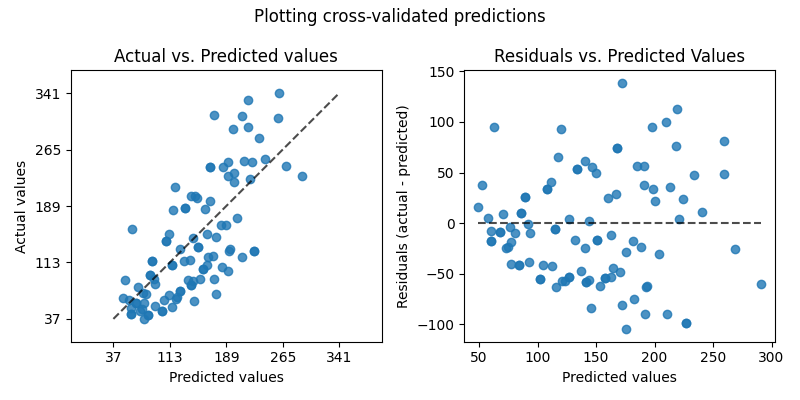
The plot on the left shows the actual values vs predicted values. For a noise-free regression task aiming to predict the (conditional) expectation of y, a perfect regression model would display data points on the diagonal defined by predicted equal to actual values. The further away from this optimal line, the larger the error of the model. In a more realistic setting with irreducible noise, that is, when not all the variations of y can be explained by features in X, then the best model would lead to a cloud of points densely arranged around the diagonal.

请注意，只有当预测值是的预期值时，上述情况才成立 y 给定 X .对于最小化均方误差目标函数或更一般地 mean Tweedie deviance 其“power”参数的任何值。

在绘制预测分位数的估计器的预测时 y 给定 X ，例如 QuantileRegressor 或任何其他模型最小化 pinball loss ，预计一小部分点位于对角线上方或下方，具体取决于估计的分位数水平。

总而言之，虽然读起来很直观，但这个情节并没有真正告诉我们如何才能获得更好的模型。

右侧图显示了剩余值（即实际值和预测值之间的差）与预测值的关系。

如果出现剩余值，则该图可以更容易地可视化 homoscedastic or heteroschedastic 分布

特别是，如果的真实分布 y|X 是Poisson或Gamma分布，预计最优模型的残余方差将随着预测值的增长 E[y|X] （对于Poisson是线性的，或者对于Gamma是二次的）。

当匹配线性最小平方回归模型时（请参阅 LinearRegression 和 Ridge ），我们可以使用这个图来检查是否有一些 model assumptions 满足，特别是残余应该不相关，其期望值应该为零，并且其方差应该是恒定的（同方差）。

如果情况并非如此，特别是如果残余图显示出一些香蕉形结构，这表明模型可能被错误指定，并且非线性特征工程或切换到非线性回归模型可能会有用。

请参阅下面的示例以查看利用此显示的模型评估。

示例

• 看到 回归模型中目标转换的效果 有关如何使用的示例 PredictionErrorDisplay 可视化学习前对目标进行转换而获得的回归模型的预测质量改进。

3.4.7. 集群指标

的 sklearn.metrics 模块实现多个损失、分数和效用函数来衡量集群性能。有关更多信息，请参阅 集群绩效评估 示例集群部分，以及 双集群评估 用于双集群化。

3.4.8. 伪估计器

在进行监督学习时，一个简单的健全性检查包括将一个人的估计量与简单的经验法则进行比较。 DummyClassifier 实现几种这样的简单分类策略：

• stratified 通过尊重训练集类别分布来生成随机预测。

• most_frequent 始终预测训练集中最频繁的标签。

• prior always predicts the class that maximizes the class prior (like most_frequent) and predict_proba returns the class prior.

• uniform 随机均匀生成预测。

• constant 始终预测用户提供的不变标签。

  这种方法的一个主要动机是F1评分，此时积极的班级是少数。

请注意，有了所有这些策略， predict 方法完全忽略输入数据！

为了说明 DummyClassifier ，首先让我们创建一个不平衡的数据集：：

>>> from sklearn.datasets import load_iris
>>> from sklearn.model_selection import train_test_split
>>> X, y = load_iris(return_X_y=True)
>>> y[y != 1] = -1
>>> X_train, X_test, y_train, y_test = train_test_split(X, y, random_state=0)

接下来，我们来比较一下 SVC 和 most_frequent

>>> from sklearn.dummy import DummyClassifier
>>> from sklearn.svm import SVC
>>> clf = SVC(kernel='linear', C=1).fit(X_train, y_train)
>>> clf.score(X_test, y_test)
0.63
>>> clf = DummyClassifier(strategy='most_frequent', random_state=0)
>>> clf.fit(X_train, y_train)
DummyClassifier(random_state=0, strategy='most_frequent')
>>> clf.score(X_test, y_test)
0.579

我们看到 SVC 并不比虚拟分类器好多少。现在，让我们更改内核：：

>>> clf = SVC(kernel='rbf', C=1).fit(X_train, y_train)
>>> clf.score(X_test, y_test)
0.94

我们看到准确率几乎提高到100%。 如果不太占用内存，建议采用交叉验证策略来更好地估计准确性。有关更多信息，请参阅 交叉验证：评估估计器性能 科.此外，如果要在参数空间上进行优化，强烈建议使用适当的方法;请参阅 调整估计器的超参数 部分了解详细信息。

更一般地说，当分类器的准确性太接近随机时，这可能意味着出现了问题：特征没有帮助、超参数没有正确调整、分类器遭受类不平衡等.

DummyRegressor 还实现了回归的四个简单经验法则：

• mean 始终预测训练目标的平均值。

• median 始终预测训练目标的中位数。

• quantile 始终预测用户提供的训练目标的分位数。

• constant 始终预测用户提供的常数值。

在所有这些策略中， predict 方法完全忽略输入数据。