使用稀疏特征对文本文档进行分类

这是一个示例，展示了如何使用scikit-learn按主题对文档进行分类 Bag of Words approach .此示例使用Tf-idf加权文档项稀疏矩阵来编码特征，并演示了可以有效处理稀疏矩阵的各种分类器。

有关通过无监督学习方法进行文档分析，请参阅示例脚本 基于k-means的文本聚类 .

# Authors: The scikit-learn developers
# SPDX-License-Identifier: BSD-3-Clause

加载并对20个新闻组文本数据集进行垂直化

我们定义了一个函数来加载数据 20个新闻组文本数据集 ，其中包括关于20个主题的约18 000个新闻组帖子，分为两个子集：一个用于培训（或发展），另一个用于测试（或绩效评估）。请注意，默认情况下，文本示例包含一些消息元数据，例如 'headers' , 'footers' （签名）和 'quotes' 到其他职位。的 fetch_20newsgroups 因此，函数接受名为 remove 试图剥离这种信息，可以使分类问题“太容易”。这是通过使用简单的算法来实现的，这些算法既不完美也不标准，因此默认情况下是禁用的。

from time import time

from sklearn.datasets import fetch_20newsgroups
from sklearn.feature_extraction.text import TfidfVectorizer

categories = [
    "alt.atheism",
    "talk.religion.misc",
    "comp.graphics",
    "sci.space",
]


def size_mb(docs):
    return sum(len(s.encode("utf-8")) for s in docs) / 1e6


def load_dataset(verbose=False, remove=()):
    """Load and vectorize the 20 newsgroups dataset."""

    data_train = fetch_20newsgroups(
        subset="train",
        categories=categories,
        shuffle=True,
        random_state=42,
        remove=remove,
    )

    data_test = fetch_20newsgroups(
        subset="test",
        categories=categories,
        shuffle=True,
        random_state=42,
        remove=remove,
    )

    # order of labels in `target_names` can be different from `categories`
    target_names = data_train.target_names

    # split target in a training set and a test set
    y_train, y_test = data_train.target, data_test.target

    # Extracting features from the training data using a sparse vectorizer
    t0 = time()
    vectorizer = TfidfVectorizer(
        sublinear_tf=True, max_df=0.5, min_df=5, stop_words="english"
    )
    X_train = vectorizer.fit_transform(data_train.data)
    duration_train = time() - t0

    # Extracting features from the test data using the same vectorizer
    t0 = time()
    X_test = vectorizer.transform(data_test.data)
    duration_test = time() - t0

    feature_names = vectorizer.get_feature_names_out()

    if verbose:
        # compute size of loaded data
        data_train_size_mb = size_mb(data_train.data)
        data_test_size_mb = size_mb(data_test.data)

        print(
            f"{len(data_train.data)} documents - "
            f"{data_train_size_mb:.2f}MB (training set)"
        )
        print(f"{len(data_test.data)} documents - {data_test_size_mb:.2f}MB (test set)")
        print(f"{len(target_names)} categories")
        print(
            f"vectorize training done in {duration_train:.3f}s "
            f"at {data_train_size_mb / duration_train:.3f}MB/s"
        )
        print(f"n_samples: {X_train.shape[0]}, n_features: {X_train.shape[1]}")
        print(
            f"vectorize testing done in {duration_test:.3f}s "
            f"at {data_test_size_mb / duration_test:.3f}MB/s"
        )
        print(f"n_samples: {X_test.shape[0]}, n_features: {X_test.shape[1]}")

    return X_train, X_test, y_train, y_test, feature_names, target_names

一种词袋文档分类器的分析

我们现在将训练分类器两次，一次在包括元数据的文本样本上训练，另一次在剥离元数据之后训练。对于这两种情况，我们将使用混淆矩阵分析测试集中的分类错误，并检查定义训练模型分类函数的系数。

没有元数据剥离的模型

我们首先使用自定义函数 load_dataset 在不剥离元数据的情况下加载数据。

X_train, X_test, y_train, y_test, feature_names, target_names = load_dataset(
    verbose=True
)

2034 documents - 3.98MB (training set)
1353 documents - 2.87MB (test set)
4 categories
vectorize training done in 0.241s at 16.502MB/s
n_samples: 2034, n_features: 7831
vectorize testing done in 0.168s at 17.040MB/s
n_samples: 1353, n_features: 7831

Our first model is an instance of the RidgeClassifier class. This is a linear classification model that uses the mean squared error on {-1, 1} encoded targets, one for each possible class. Contrary to LogisticRegression, RidgeClassifier does not provide probabilistic predictions (no predict_proba method), but it is often faster to train.

from sklearn.linear_model import RidgeClassifier

clf = RidgeClassifier(tol=1e-2, solver="sparse_cg")
clf.fit(X_train, y_train)
pred = clf.predict(X_test)

我们绘制这个分类器的混淆矩阵，以确定分类错误中是否存在模式。

import matplotlib.pyplot as plt

from sklearn.metrics import ConfusionMatrixDisplay

fig, ax = plt.subplots(figsize=(10, 5))
ConfusionMatrixDisplay.from_predictions(y_test, pred, ax=ax)
ax.xaxis.set_ticklabels(target_names)
ax.yaxis.set_ticklabels(target_names)
_ = ax.set_title(
    f"Confusion Matrix for {clf.__class__.__name__}\non the original documents"
)

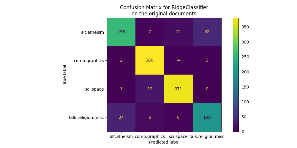
混淆矩阵强调， alt.atheism 类经常与类文档混淆 talk.religion.misc 类，反之亦然，这是意料之中的，因为主题在语义上是相关的。

我们还观察到一些文件 sci.space 类可能被错误分类为 comp.graphics 而相反的情况则要罕见得多。需要对这些严重机密的文件进行手动检查，才能深入了解这种不对称性。空间主题的词汇可能比计算机图形的词汇更具体。

我们可以通过查看平均特征效应最高的单词来更深入地了解这个分类器如何做出决策：

import numpy as np
import pandas as pd


def plot_feature_effects():
    # learned coefficients weighted by frequency of appearance
    average_feature_effects = clf.coef_ * np.asarray(X_train.mean(axis=0)).ravel()

    for i, label in enumerate(target_names):
        top5 = np.argsort(average_feature_effects[i])[-5:][::-1]
        if i == 0:
            top = pd.DataFrame(feature_names[top5], columns=[label])
            top_indices = top5
        else:
            top[label] = feature_names[top5]
            top_indices = np.concatenate((top_indices, top5), axis=None)
    top_indices = np.unique(top_indices)
    predictive_words = feature_names[top_indices]

    # plot feature effects
    bar_size = 0.25
    padding = 0.75
    y_locs = np.arange(len(top_indices)) * (4 * bar_size + padding)

    fig, ax = plt.subplots(figsize=(10, 8))
    for i, label in enumerate(target_names):
        ax.barh(
            y_locs + (i - 2) * bar_size,
            average_feature_effects[i, top_indices],
            height=bar_size,
            label=label,
        )
    ax.set(
        yticks=y_locs,
        yticklabels=predictive_words,
        ylim=[
            0 - 4 * bar_size,
            len(top_indices) * (4 * bar_size + padding) - 4 * bar_size,
        ],
    )
    ax.legend(loc="lower right")

    print("top 5 keywords per class:")
    print(top)

    return ax


_ = plot_feature_effects().set_title("Average feature effect on the original data")

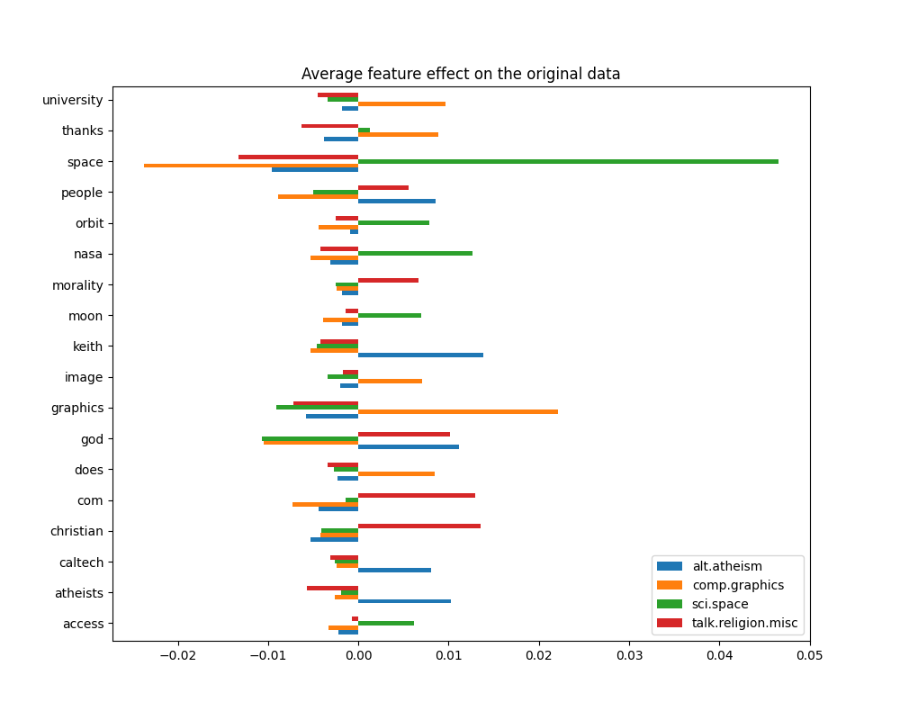
top 5 keywords per class:
  alt.atheism comp.graphics sci.space talk.religion.misc
0       keith      graphics     space          christian
1         god    university      nasa                com
2    atheists        thanks     orbit                god
3      people          does      moon           morality
4     caltech         image    access             people

我们可以观察到，最具预测性的词通常与单个类别呈强正相关，而与所有其他类别呈负相关。大多数积极的联系都很容易解释。然而，有些词，例如 "god" 和 "people" 与两者正相关 "talk.misc.religion" 和 "alt.atheism" 因为这两个类共享一些共同的词汇。但请注意，还有诸如此类的词语 "christian" 和 "morality" 仅与之正相关 "talk.misc.religion" .此外，在此版本的数据集中， "caltech" 由于数据集的污染来自某种元数据，例如讨论中之前电子邮件发件人的电子邮件地址，因此是无神论的首要预测特征之一，如下所示：

data_train = fetch_20newsgroups(
    subset="train", categories=categories, shuffle=True, random_state=42
)

for doc in data_train.data:
    if "caltech" in doc:
        print(doc)
        break

From: livesey@solntze.wpd.sgi.com (Jon Livesey)
Subject: Re: Morality? (was Re: <Political Atheists?)
Organization: sgi
Lines: 93
Distribution: world
NNTP-Posting-Host: solntze.wpd.sgi.com

In article <1qlettINN8oi@gap.caltech.edu>, keith@cco.caltech.edu (Keith Allan Schneider) writes:
|> livesey@solntze.wpd.sgi.com (Jon Livesey) writes:
|>
|> >>>Explain to me
|> >>>how instinctive acts can be moral acts, and I am happy to listen.
|> >>For example, if it were instinctive not to murder...
|> >
|> >Then not murdering would have no moral significance, since there
|> >would be nothing voluntary about it.
|>
|> See, there you go again, saying that a moral act is only significant
|> if it is "voluntary."  Why do you think this?

If you force me to do something, am I morally responsible for it?

|>
|> And anyway, humans have the ability to disregard some of their instincts.

Well, make up your mind.    Is it to be "instinctive not to murder"
or not?

|>
|> >>So, only intelligent beings can be moral, even if the bahavior of other
|> >>beings mimics theirs?
|> >
|> >You are starting to get the point.  Mimicry is not necessarily the
|> >same as the action being imitated.  A Parrot saying "Pretty Polly"
|> >isn't necessarily commenting on the pulchritude of Polly.
|>
|> You are attaching too many things to the term "moral," I think.
|> Let's try this:  is it "good" that animals of the same species
|> don't kill each other.  Or, do you think this is right?

It's not even correct.    Animals of the same species do kill
one another.

|>
|> Or do you think that animals are machines, and that nothing they do
|> is either right nor wrong?

Sigh.   I wonder how many times we have been round this loop.

I think that instinctive bahaviour has no moral significance.
I am quite prepared to believe that higher animals, such as
primates, have the beginnings of a moral sense, since they seem
to exhibit self-awareness.

|>
|>
|> >>Animals of the same species could kill each other arbitarily, but
|> >>they don't.
|> >
|> >They do.  I and other posters have given you many examples of exactly
|> >this, but you seem to have a very short memory.
|>
|> Those weren't arbitrary killings.  They were slayings related to some
|> sort of mating ritual or whatnot.

So what?     Are you trying to say that some killing in animals
has a moral significance and some does not?   Is this your
natural morality>


|>
|> >>Are you trying to say that this isn't an act of morality because
|> >>most animals aren't intelligent enough to think like we do?
|> >
|> >I'm saying:
|> >    "There must be the possibility that the organism - it's not
|> >    just people we are talking about - can consider alternatives."
|> >
|> >It's right there in the posting you are replying to.
|>
|> Yes it was, but I still don't understand your distinctions.  What
|> do you mean by "consider?"  Can a small child be moral?  How about
|> a gorilla?  A dolphin?  A platypus?  Where is the line drawn?  Does
|> the being need to be self aware?

Are you blind?   What do you think that this sentence means?

        "There must be the possibility that the organism - it's not
        just people we are talking about - can consider alternatives."

What would that imply?

|>
|> What *do* you call the mechanism which seems to prevent animals of
|> the same species from (arbitrarily) killing each other?  Don't
|> you find the fact that they don't at all significant?

I find the fact that they do to be significant.

jon.

此类标题、签名页脚（以及引用的之前消息的元数据）可以被视为辅助信息，通过识别注册成员来人为地揭示新闻组，并且人们宁愿希望我们的文本分类器只从每个文本文档的“主要内容”中学习，而不是依赖于泄露的作家身份。

带元数据剥离的模型

的 remove scikit-learn中的20个新闻组数据集加载器选项允许尝试过滤掉一些不需要的元数据，从而人为地使分类问题变得更容易。请注意，这种对文本内容的过滤远非完美。

让我们尝试利用此选项来训练文本分类器，该分类器不会过多依赖此类元数据来做出决策：

(
    X_train,
    X_test,
    y_train,
    y_test,
    feature_names,
    target_names,
) = load_dataset(remove=("headers", "footers", "quotes"))

clf = RidgeClassifier(tol=1e-2, solver="sparse_cg")
clf.fit(X_train, y_train)
pred = clf.predict(X_test)

fig, ax = plt.subplots(figsize=(10, 5))
ConfusionMatrixDisplay.from_predictions(y_test, pred, ax=ax)
ax.xaxis.set_ticklabels(target_names)
ax.yaxis.set_ticklabels(target_names)
_ = ax.set_title(
    f"Confusion Matrix for {clf.__class__.__name__}\non filtered documents"
)

通过查看混淆矩阵，可以更明显地看出，用元数据训练的模型的分数过于乐观。不访问元数据的分类问题不太准确，但更能代表预期的文本分类问题。

_ = plot_feature_effects().set_title("Average feature effects on filtered documents")

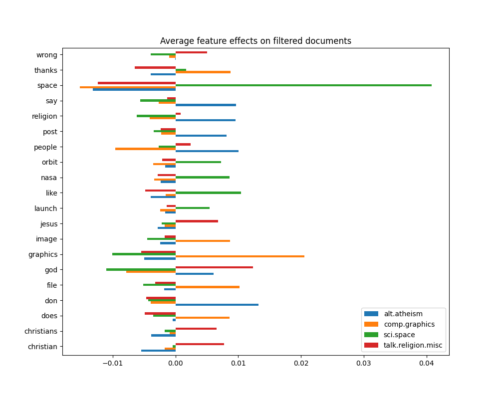
top 5 keywords per class:
  alt.atheism comp.graphics sci.space talk.religion.misc
0         don      graphics     space                god
1      people          file      like          christian
2         say        thanks      nasa              jesus
3    religion         image     orbit         christians
4        post          does    launch              wrong

在下一部分中，我们保留不带元数据的数据集来比较几个分类器。

基准分类器

Scikit-learn提供了许多不同类型的分类算法。在本节中，我们将针对同一文本分类问题训练精选的分类器，并在训练时和测试时测量它们的概括性能（测试集的准确性）和计算性能（速度）。为此目的，我们定义了以下基准实用程序：

from sklearn import metrics
from sklearn.utils.extmath import density


def benchmark(clf, custom_name=False):
    print("_" * 80)
    print("Training: ")
    print(clf)
    t0 = time()
    clf.fit(X_train, y_train)
    train_time = time() - t0
    print(f"train time: {train_time:.3}s")

    t0 = time()
    pred = clf.predict(X_test)
    test_time = time() - t0
    print(f"test time:  {test_time:.3}s")

    score = metrics.accuracy_score(y_test, pred)
    print(f"accuracy:   {score:.3}")

    if hasattr(clf, "coef_"):
        print(f"dimensionality: {clf.coef_.shape[1]}")
        print(f"density: {density(clf.coef_)}")
        print()

    print()
    if custom_name:
        clf_descr = str(custom_name)
    else:
        clf_descr = clf.__class__.__name__
    return clf_descr, score, train_time, test_time

我们现在使用8个不同的分类模型训练和测试数据集，并获得每个模型的性能结果。本研究的目标是强调不同类型分类器对于此类多类文本分类问题的计算/准确性权衡。

请注意，最重要的超参数值是使用网格搜索过程进行调整的，为了简单起见，本笔记本中没有显示。查看示例脚本 用于文本特征提取和评估的样本管道 # noqa：E501，演示如何进行此类调整。

from sklearn.ensemble import RandomForestClassifier
from sklearn.linear_model import LogisticRegression, SGDClassifier
from sklearn.naive_bayes import ComplementNB
from sklearn.neighbors import KNeighborsClassifier, NearestCentroid
from sklearn.svm import LinearSVC

results = []
for clf, name in (
    (LogisticRegression(C=5, max_iter=1000), "Logistic Regression"),
    (RidgeClassifier(alpha=1.0, solver="sparse_cg"), "Ridge Classifier"),
    (KNeighborsClassifier(n_neighbors=100), "kNN"),
    (RandomForestClassifier(), "Random Forest"),
    # L2 penalty Linear SVC
    (LinearSVC(C=0.1, dual=False, max_iter=1000), "Linear SVC"),
    # L2 penalty Linear SGD
    (
        SGDClassifier(
            loss="log_loss", alpha=1e-4, n_iter_no_change=3, early_stopping=True
        ),
        "log-loss SGD",
    ),
    # NearestCentroid (aka Rocchio classifier)
    (NearestCentroid(), "NearestCentroid"),
    # Sparse naive Bayes classifier
    (ComplementNB(alpha=0.1), "Complement naive Bayes"),
):
    print("=" * 80)
    print(name)
    results.append(benchmark(clf, name))

================================================================================
Logistic Regression
________________________________________________________________________________
Training:
LogisticRegression(C=5, max_iter=1000)
train time: 0.648s
test time:  0.00211s
accuracy:   0.772
dimensionality: 5316
density: 1.0


================================================================================
Ridge Classifier
________________________________________________________________________________
Training:
RidgeClassifier(solver='sparse_cg')
train time: 0.0476s
test time:  0.000831s
accuracy:   0.76
dimensionality: 5316
density: 1.0


================================================================================
kNN
________________________________________________________________________________
Training:
KNeighborsClassifier(n_neighbors=100)
train time: 0.000809s
test time:  0.0677s
accuracy:   0.752

================================================================================
Random Forest
________________________________________________________________________________
Training:
RandomForestClassifier()
train time: 1.19s
test time:  0.0434s
accuracy:   0.7

================================================================================
Linear SVC
________________________________________________________________________________
Training:
LinearSVC(C=0.1, dual=False)
train time: 0.0238s
test time:  0.000496s
accuracy:   0.752
dimensionality: 5316
density: 1.0


================================================================================
log-loss SGD
________________________________________________________________________________
Training:
SGDClassifier(early_stopping=True, loss='log_loss', n_iter_no_change=3)
train time: 0.0251s
test time:  0.000581s
accuracy:   0.764
dimensionality: 5316
density: 1.0


================================================================================
NearestCentroid
________________________________________________________________________________
Training:
NearestCentroid()
train time: 0.116s
test time:  0.00258s
accuracy:   0.748

================================================================================
Complement naive Bayes
________________________________________________________________________________
Training:
ComplementNB(alpha=0.1)
train time: 0.00144s
test time:  0.000561s
accuracy:   0.779

绘制每个分类器的准确性、训练和测试时间

散点图显示了每个分类器的测试精度与训练和测试时间之间的权衡。

indices = np.arange(len(results))

results = [[x[i] for x in results] for i in range(4)]

clf_names, score, training_time, test_time = results
training_time = np.array(training_time)
test_time = np.array(test_time)

fig, ax1 = plt.subplots(figsize=(10, 8))
ax1.scatter(score, training_time, s=60)
ax1.set(
    title="Score-training time trade-off",
    yscale="log",
    xlabel="test accuracy",
    ylabel="training time (s)",
)
fig, ax2 = plt.subplots(figsize=(10, 8))
ax2.scatter(score, test_time, s=60)
ax2.set(
    title="Score-test time trade-off",
    yscale="log",
    xlabel="test accuracy",
    ylabel="test time (s)",
)

for i, txt in enumerate(clf_names):
    ax1.annotate(txt, (score[i], training_time[i]))
    ax2.annotate(txt, (score[i], test_time[i]))

• 
• 

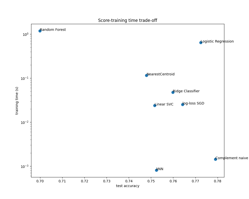
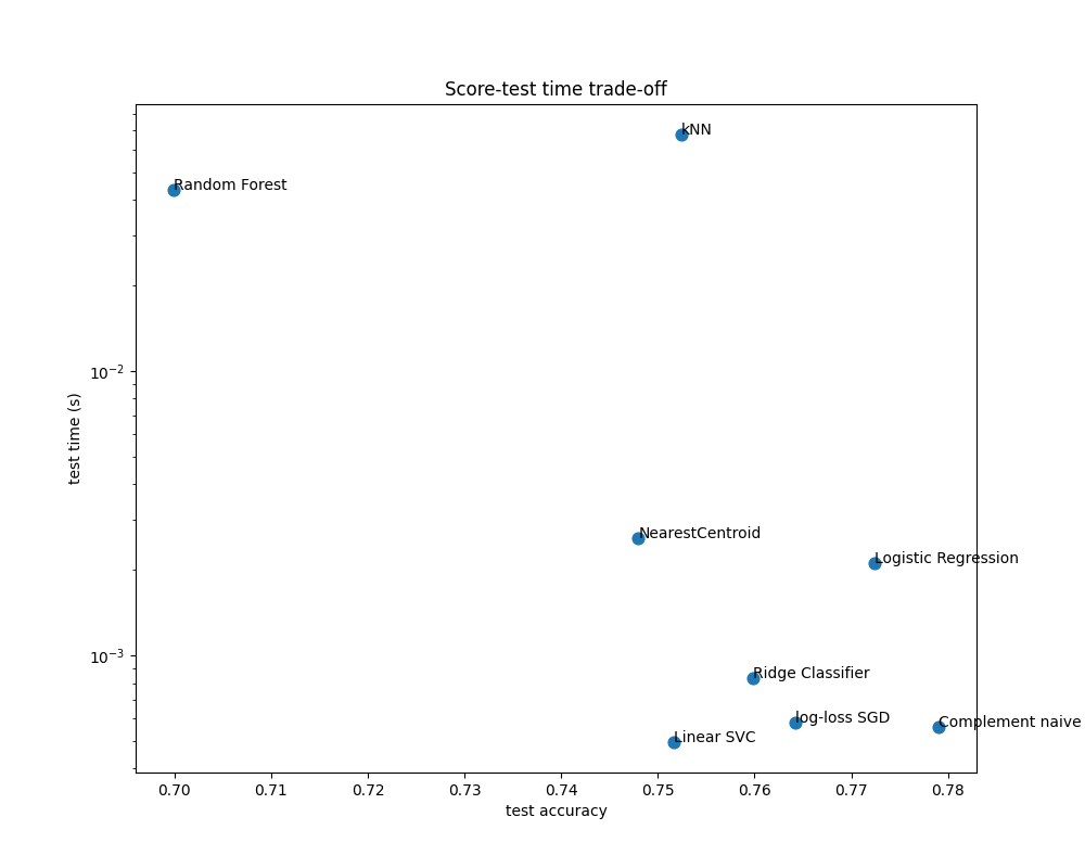
朴素的Bayes模型在分数和训练/测试时间之间具有最佳的权衡，而Random Forest模型训练速度慢、预测成本高且准确性相对较差。预计这是：对于多维预测问题，线性模型通常更适合，因为当特征空间具有10，000个或更多维度时，大多数问题变得线性可分离。

线性模型训练速度和准确性的差异可以通过优化的损失函数的选择和使用的正规化类型来解释。请注意，一些损失相同但求解器或正规化配置不同的线性模型可能会产生不同的适配时间和测试准确性。我们可以在第二个图中观察到，一旦训练，所有线性模型都具有大致相同的预测速度，这是预期的，因为它们都实现了相同的预测功能。

KNeighborsClassifier的准确性相对较低，但测试时间最长。预测时间也很长：对于每次预测，模型必须计算测试样本和训练集中每个文档之间的成对距离，这在计算上很昂贵。此外，“维度诅咒”损害了该模型在文本分类问题的多维特征空间中产生竞争准确性的能力。

相关实例

用于文本特征提取和评估的样本管道

Sample pipeline for text feature extraction and evaluation

使用谱协同集群算法对文档进行二集群

Biclustering documents with the Spectral Co-clustering algorithm

基于k-means的文本聚类

Clustering text documents using k-means

收件箱Hasher和DictVectorizer比较

FeatureHasher and DictVectorizer Comparison