可视化VotingClassifier的概率预测#

在玩具数据集中绘制预测类别概率，由三个不同的分类器预测并由 VotingClassifier .

首先，初始化三个线性分类器。两种是具有相互作用项的样条模型，一种使用恒定外推，另一种使用周期外推。第三个分类器是 Nystroem 使用默认的“rBF”内核。

在本示例的第一部分中，这三个分类器用于演示软投票 VotingClassifier 加权平均值。我们设定 weights=[2, 1, 3] 这意味着恒外推样条模型的预测的加权是周期样条模型的两倍，而Nystroem模型的预测的加权是周期样条的三倍。

第二部分演示了如何将软预测转化为硬预测。

# Authors: The scikit-learn developers
# SPDX-License-Identifier: BSD-3-Clause

我们首先生成一个有噪的异或数据集，这是一个二进制分类任务。

import matplotlib.pyplot as plt
import numpy as np
import pandas as pd
from matplotlib.colors import ListedColormap

n_samples = 500
rng = np.random.default_rng(0)
feature_names = ["Feature #0", "Feature #1"]
common_scatter_plot_params = dict(
    cmap=ListedColormap(["tab:red", "tab:blue"]),
    edgecolor="white",
    linewidth=1,
)

xor = pd.DataFrame(
    np.random.RandomState(0).uniform(low=-1, high=1, size=(n_samples, 2)),
    columns=feature_names,
)
noise = rng.normal(loc=0, scale=0.1, size=(n_samples, 2))
target_xor = np.logical_xor(
    xor["Feature #0"] + noise[:, 0] > 0, xor["Feature #1"] + noise[:, 1] > 0
)

X = xor[feature_names]
y = target_xor.astype(np.int32)

fig, ax = plt.subplots()
ax.scatter(X["Feature #0"], X["Feature #1"], c=y, **common_scatter_plot_params)
ax.set_title("The XOR dataset")
plt.show()

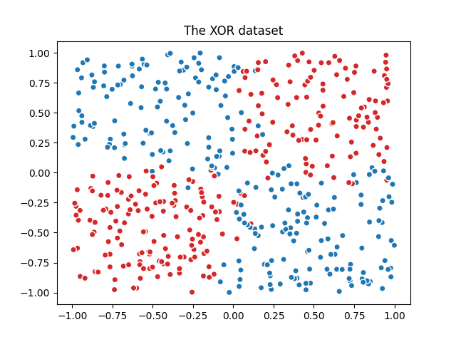
由于异或数据集固有的非线性可分离性，通常更喜欢基于树的模型。然而，适当的特征工程与线性模型相结合可以产生有效的结果，并且还可以为位于受噪音影响的过渡区域中的样本产生更好校准的概率。

我们在整个数据集上定义并匹配模型。

from sklearn.ensemble import VotingClassifier
from sklearn.kernel_approximation import Nystroem
from sklearn.linear_model import LogisticRegression
from sklearn.pipeline import make_pipeline
from sklearn.preprocessing import PolynomialFeatures, SplineTransformer, StandardScaler

clf1 = make_pipeline(
    SplineTransformer(degree=2, n_knots=2),
    PolynomialFeatures(interaction_only=True),
    LogisticRegression(C=10),
)
clf2 = make_pipeline(
    SplineTransformer(
        degree=2,
        n_knots=4,
        extrapolation="periodic",
        include_bias=True,
    ),
    PolynomialFeatures(interaction_only=True),
    LogisticRegression(C=10),
)
clf3 = make_pipeline(
    StandardScaler(),
    Nystroem(gamma=2, random_state=0),
    LogisticRegression(C=10),
)
weights = [2, 1, 3]
eclf = VotingClassifier(
    estimators=[
        ("constant splines model", clf1),
        ("periodic splines model", clf2),
        ("nystroem model", clf3),
    ],
    voting="soft",
    weights=weights,
)

clf1.fit(X, y)
clf2.fit(X, y)
clf3.fit(X, y)
eclf.fit(X, y)

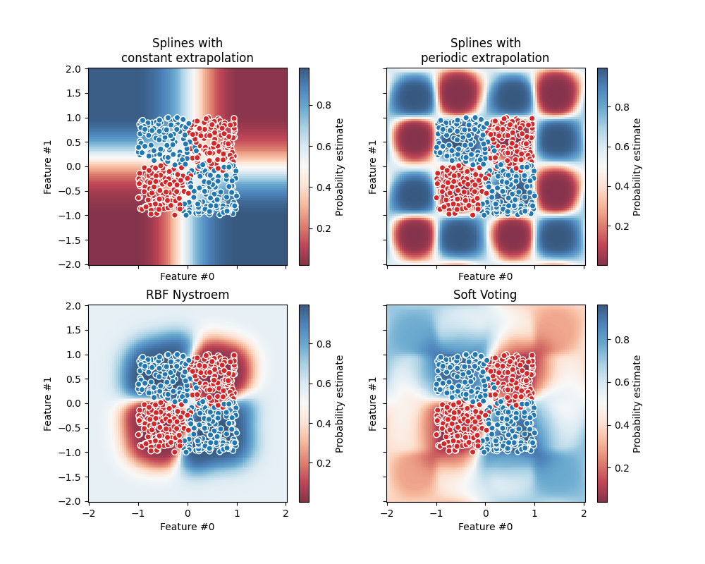
最后利用 DecisionBoundaryDisplay 来绘制预测概率。通过使用发散的色彩映射表（例如 "RdBu" ），我们可以确保深色对应于 predict_proba 接近0或1，白色对应于 predict_proba 的0.5。

from itertools import product

from sklearn.inspection import DecisionBoundaryDisplay

fig, axarr = plt.subplots(2, 2, sharex="col", sharey="row", figsize=(10, 8))
for idx, clf, title in zip(
    product([0, 1], [0, 1]),
    [clf1, clf2, clf3, eclf],
    [
        "Splines with\nconstant extrapolation",
        "Splines with\nperiodic extrapolation",
        "RBF Nystroem",
        "Soft Voting",
    ],
):
    disp = DecisionBoundaryDisplay.from_estimator(
        clf,
        X,
        response_method="predict_proba",
        plot_method="pcolormesh",
        cmap="RdBu",
        alpha=0.8,
        ax=axarr[idx[0], idx[1]],
    )
    axarr[idx[0], idx[1]].scatter(
        X["Feature #0"],
        X["Feature #1"],
        c=y,
        **common_scatter_plot_params,
    )
    axarr[idx[0], idx[1]].set_title(title)
    fig.colorbar(disp.surface_, ax=axarr[idx[0], idx[1]], label="Probability estimate")

plt.show()

Splines with constant extrapolation, Splines with periodic extrapolation, RBF Nystroem, Soft Voting

作为健全性检查，我们可以为给定样本验证 VotingClassifier 确实是各个分类器软预测的加权平均值。

在本示例中的二元分类的情况下， predict_proba 数组包含属于类0的概率（这里用红色表示）作为第一个条目，属于类1的概率（这里用蓝色表示）作为第二个条目。

test_sample = pd.DataFrame({"Feature #0": [-0.5], "Feature #1": [1.5]})
predict_probas = [est.predict_proba(test_sample).ravel() for est in eclf.estimators_]
for (est_name, _), est_probas in zip(eclf.estimators, predict_probas):
    print(f"{est_name}'s predicted probabilities: {est_probas}")

constant splines model's predicted probabilities: [0.11272662 0.88727338]
periodic splines model's predicted probabilities: [0.99726573 0.00273427]
nystroem model's predicted probabilities: [0.3185838 0.6814162]

print(
    "Weighted average of soft-predictions: "
    f"{np.dot(weights, predict_probas) / np.sum(weights)}"
)

Weighted average of soft-predictions: [0.3630784 0.6369216]

我们可以看到，上面手动计算的预测概率相当于 VotingClassifier :

print(
    "Predicted probability of VotingClassifier: "
    f"{eclf.predict_proba(test_sample).ravel()}"
)

Predicted probability of VotingClassifier: [0.3630784 0.6369216]

为了在提供权重时将软预测转换为硬预测，需要为每个类别计算加权平均预测概率。然后，从平均概率最高的类别标签中推导出最终的类别标签，其对应于默认阈值 predict_proba=0.5 在二元分类的情况下。

print(
    "Class with the highest weighted average of soft-predictions: "
    f"{np.argmax(np.dot(weights, predict_probas) / np.sum(weights))}"
)

Class with the highest weighted average of soft-predictions: 1

这相当于 VotingClassifier 的 predict 方法：

print(f"Predicted class of VotingClassifier: {eclf.predict(test_sample).ravel()}")

Predicted class of VotingClassifier: [1]

软投票可以像任何其他概率分类器一样进行阈值化。这允许您设置预测阳性类别的阈值概率，而不是简单地选择预测概率最高的类别。

from sklearn.model_selection import FixedThresholdClassifier

eclf_other_threshold = FixedThresholdClassifier(
    eclf, threshold=0.7, response_method="predict_proba"
).fit(X, y)
print(
    "Predicted class of thresholded VotingClassifier: "
    f"{eclf_other_threshold.predict(test_sample)}"
)

Predicted class of thresholded VotingClassifier: [0]

Total running time of the script: （0分0.594秒）