具有显示对象的可视化#

在这个例子中，我们将构建显示对象， ConfusionMatrixDisplay , RocCurveDisplay ，而且 PrecisionRecallDisplay 直接来自他们各自的指标。当模型的预测已经计算或计算成本很高时，这是使用相应图函数的替代方案。请注意，这是高级用途，一般来说，我们建议使用它们各自的绘图功能。

# Authors: The scikit-learn developers
# SPDX-License-Identifier: BSD-3-Clause

负载数据和列车模型#

对于本例，我们加载输血服务中心数据集 OpenML .这是一个二元分类问题，目标是个人是否献血。然后将数据分成训练和测试数据集，并将逻辑回归与训练数据集进行匹配。

from sklearn.datasets import fetch_openml
from sklearn.linear_model import LogisticRegression
from sklearn.model_selection import train_test_split
from sklearn.pipeline import make_pipeline
from sklearn.preprocessing import StandardScaler

X, y = fetch_openml(data_id=1464, return_X_y=True)
X_train, X_test, y_train, y_test = train_test_split(X, y, stratify=y)

clf = make_pipeline(StandardScaler(), LogisticRegression(random_state=0))
clf.fit(X_train, y_train)

Pipeline(steps=[('standardscaler', StandardScaler()),
                ('logisticregression', LogisticRegression(random_state=0))])

In a Jupyter environment, please rerun this cell to show the HTML representation or trust the notebook.
On GitHub, the HTML representation is unable to render, please try loading this page with nbviewer.org.

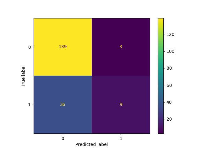
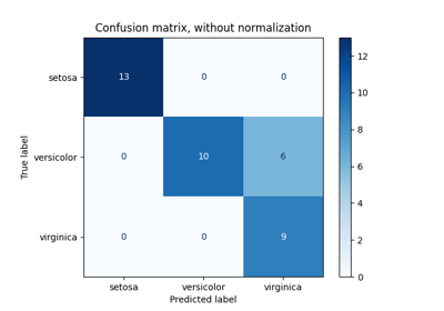
创建 `ConfusionMatrixDisplay`#

使用拟合模型，我们计算模型在测试数据集上的预测。这些预测用于计算混淆矩阵，该混淆矩阵用 ConfusionMatrixDisplay

from sklearn.metrics import ConfusionMatrixDisplay, confusion_matrix

y_pred = clf.predict(X_test)
cm = confusion_matrix(y_test, y_pred)

cm_display = ConfusionMatrixDisplay(cm).plot()

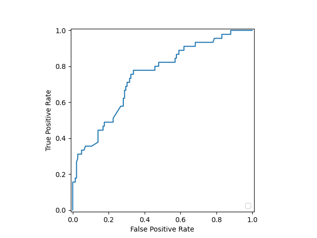
创建 `RocCurveDisplay`#

roc曲线需要来自估计器的概率或非阈值决策值。由于逻辑回归提供了决策函数，因此我们将使用它来绘制roc曲线：

from sklearn.metrics import RocCurveDisplay, roc_curve

y_score = clf.decision_function(X_test)

fpr, tpr, _ = roc_curve(y_test, y_score, pos_label=clf.classes_[1])
roc_display = RocCurveDisplay(fpr=fpr, tpr=tpr).plot()

/xpy/lib/python3.11/site-packages/sklearn/metrics/_plot/roc_curve.py:189: UserWarning:

No artists with labels found to put in legend.  Note that artists whose label start with an underscore are ignored when legend() is called with no argument.

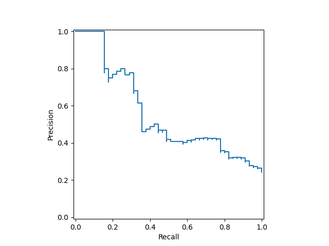
创建 `PrecisionRecallDisplay`#

类似地，精确召回曲线可以使用 y_score 从预视部分。

from sklearn.metrics import PrecisionRecallDisplay, precision_recall_curve

prec, recall, _ = precision_recall_curve(y_test, y_score, pos_label=clf.classes_[1])
pr_display = PrecisionRecallDisplay(precision=prec, recall=recall).plot()

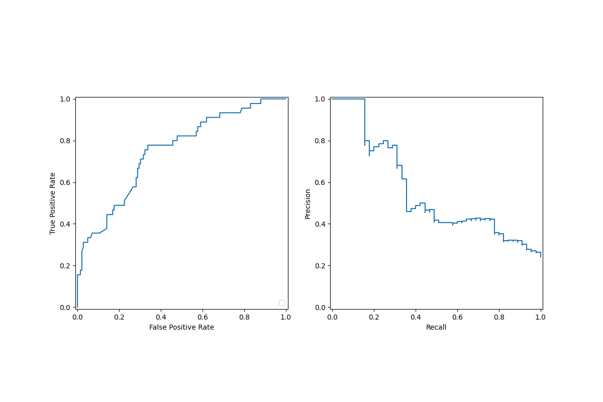
将显示对象组合到单个地块中#

显示对象存储作为参数传递的计算值。这使得可以使用matplotlib的API轻松组合可视化。在下面的示例中，我们将显示器并排放置在一行中。

import matplotlib.pyplot as plt

fig, (ax1, ax2) = plt.subplots(1, 2, figsize=(12, 8))

roc_display.plot(ax=ax1)
pr_display.plot(ax=ax2)
plt.show()

/xpy/lib/python3.11/site-packages/sklearn/metrics/_plot/roc_curve.py:189: UserWarning:

No artists with labels found to put in legend.  Note that artists whose label start with an underscore are ignored when legend() is called with no argument.

Total running time of the script: （0分0.255秒）