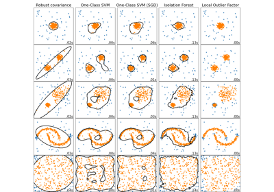
隔离森林示例#

示例的使用 IsolationForest 用于异常检测

的孤立森林是“隔离树”的集合，通过循环随机划分来“隔离”观察结果，可以用树结构来表示。对于离群值，分离样本所需的分裂次数较低，对于内值则较高。

在本示例中，我们演示了两种可视化在玩具数据集上训练的隔离森林决策边界的方法。

# Authors: The scikit-learn developers
# SPDX-License-Identifier: BSD-3-Clause

数据生成#

我们生成两个集群（每个集群包含 n_samples ）通过随机抽样返回的标准正态分布 numpy.random.randn .其中一个是球形的，另一个轻微变形。

为了与 IsolationForest 符号时，内点（即高斯集群）被分配一个地面真值标签 1 而异常值（由 numpy.random.uniform ）被赋予标签 -1 .

import numpy as np

from sklearn.model_selection import train_test_split

n_samples, n_outliers = 120, 40
rng = np.random.RandomState(0)
covariance = np.array([[0.5, -0.1], [0.7, 0.4]])
cluster_1 = 0.4 * rng.randn(n_samples, 2) @ covariance + np.array([2, 2])  # general
cluster_2 = 0.3 * rng.randn(n_samples, 2) + np.array([-2, -2])  # spherical
outliers = rng.uniform(low=-4, high=4, size=(n_outliers, 2))

X = np.concatenate([cluster_1, cluster_2, outliers])
y = np.concatenate(
    [np.ones((2 * n_samples), dtype=int), -np.ones((n_outliers), dtype=int)]
)

X_train, X_test, y_train, y_test = train_test_split(X, y, stratify=y, random_state=42)

我们可以可视化得到的集群：

import matplotlib.pyplot as plt

scatter = plt.scatter(X[:, 0], X[:, 1], c=y, s=20, edgecolor="k")
handles, labels = scatter.legend_elements()
plt.axis("square")
plt.legend(handles=handles, labels=["outliers", "inliers"], title="true class")
plt.title("Gaussian inliers with \nuniformly distributed outliers")
plt.show()

Gaussian inliers with uniformly distributed outliers

训练模型#

from sklearn.ensemble import IsolationForest

clf = IsolationForest(max_samples=100, random_state=0)
clf.fit(X_train)

IsolationForest(max_samples=100, random_state=0)

In a Jupyter environment, please rerun this cell to show the HTML representation or trust the notebook.
On GitHub, the HTML representation is unable to render, please try loading this page with nbviewer.org.

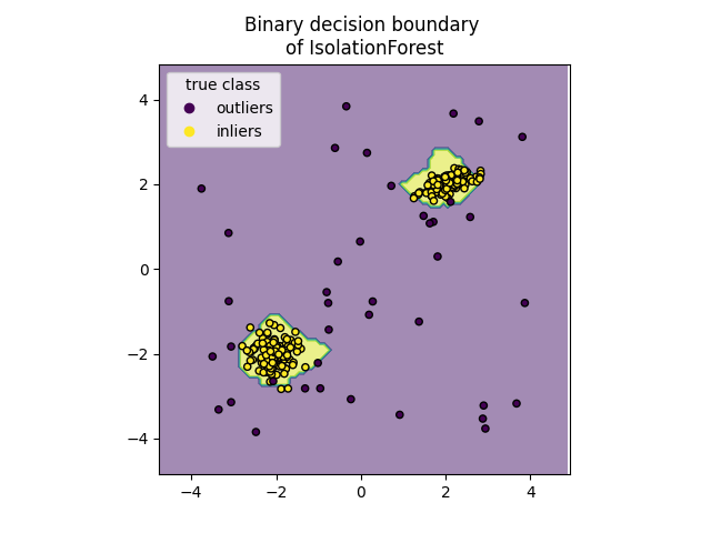
绘制离散决策边界#

我们使用类 DecisionBoundaryDisplay 可视化离散的决策边界。背景颜色表示该给定区域中的样本是否被预测为异常值。散点图显示真实标签。

import matplotlib.pyplot as plt

from sklearn.inspection import DecisionBoundaryDisplay

disp = DecisionBoundaryDisplay.from_estimator(
    clf,
    X,
    response_method="predict",
    alpha=0.5,
)
disp.ax_.scatter(X[:, 0], X[:, 1], c=y, s=20, edgecolor="k")
disp.ax_.set_title("Binary decision boundary \nof IsolationForest")
plt.axis("square")
plt.legend(handles=handles, labels=["outliers", "inliers"], title="true class")
plt.show()

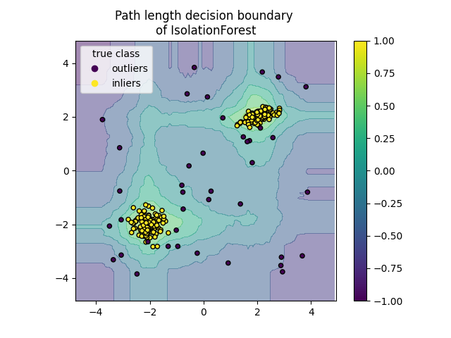
Binary decision boundary of IsolationForest

地块路径长度决策边界#

通过设置 response_method="decision_function" ，的背景 DecisionBoundaryDisplay 代表观察结果的正常性测量。这样的分数是由随机树木森林上平均的路径长度给出的，而路径长度本身是由隔离给定样本所需的叶子深度（或相当于分裂的数量）给出的。

当随机树森林集体产生用于隔离一些特定样本的短路径长度时，它们很可能是异常，并且正态性的测量接近 0 .同样，大路径对应于接近 1 并且更有可能是内亲。

disp = DecisionBoundaryDisplay.from_estimator(
    clf,
    X,
    response_method="decision_function",
    alpha=0.5,
)
disp.ax_.scatter(X[:, 0], X[:, 1], c=y, s=20, edgecolor="k")
disp.ax_.set_title("Path length decision boundary \nof IsolationForest")
plt.axis("square")
plt.legend(handles=handles, labels=["outliers", "inliers"], title="true class")
plt.colorbar(disp.ax_.collections[1])
plt.show()

Path length decision boundary of IsolationForest

Total running time of the script: （0分0.331秒）