事后调整决策函数的截止点#

一旦训练了二元分类器， predict 方法输出对应于 decision_function 或 predict_proba 输出.默认阈值定义为后验概率估计0.5或决策分数0.0。然而，这种默认策略对于手头的任务来说可能不是最佳的。

此示例展示了如何使用 TunedThresholdClassifierCV 根据感兴趣的指标调整决策阈值。

# Authors: The scikit-learn developers
# SPDX-License-Identifier: BSD-3-Clause

糖尿病数据集#

为了说明决策阈值的调整，我们将使用糖尿病数据集。该数据集可在OpenML上获取：https://www.openml.org/d/37。公司现采用国际 fetch_openml 函数获取此数据集。

from sklearn.datasets import fetch_openml

diabetes = fetch_openml(data_id=37, as_frame=True, parser="pandas")
data, target = diabetes.data, diabetes.target

我们查看目标以了解我们正在处理的问题类型。

target.value_counts()

class
tested_negative    500
tested_positive    268
Name: count, dtype: int64

我们可以看到我们正在处理一个二元分类问题。由于标签没有编码为0和1，因此我们明确表示，我们将标记为“tested_negative”的类视为负类（这也是最常见的），将标记为“tested_negative”的类视为正类：

neg_label, pos_label = target.value_counts().index

我们还可以观察到，这个二元问题是稍微不平衡的，我们有大约两倍多的样本来自负类比来自正类。当谈到评价时，我们应该考虑这方面来解释结果。

我们的香草分类器#

我们定义了一个基本的预测模型，该模型由缩放器和逻辑回归分类器组成。

from sklearn.linear_model import LogisticRegression
from sklearn.pipeline import make_pipeline
from sklearn.preprocessing import StandardScaler

model = make_pipeline(StandardScaler(), LogisticRegression())
model

Pipeline(steps=[('standardscaler', StandardScaler()),
                ('logisticregression', LogisticRegression())])

In a Jupyter environment, please rerun this cell to show the HTML representation or trust the notebook.
On GitHub, the HTML representation is unable to render, please try loading this page with nbviewer.org.

我们使用交叉验证来评估我们的模型。我们使用准确度和平衡准确度来报告模型的性能。平衡准确度是一个对类不平衡不太敏感的指标，它将允许我们正确看待准确度得分。

交叉验证使我们能够研究不同数据分割之间决策阈值的方差。然而，数据集相当小，使用超过5倍来评估分散度是有害的。因此，我们使用 RepeatedStratifiedKFold 其中我们应用5重交叉验证的几次重复。

import pandas as pd

from sklearn.model_selection import RepeatedStratifiedKFold, cross_validate

scoring = ["accuracy", "balanced_accuracy"]
cv_scores = [
    "train_accuracy",
    "test_accuracy",
    "train_balanced_accuracy",
    "test_balanced_accuracy",
]
cv = RepeatedStratifiedKFold(n_splits=5, n_repeats=10, random_state=42)
cv_results_vanilla_model = pd.DataFrame(
    cross_validate(
        model,
        data,
        target,
        scoring=scoring,
        cv=cv,
        return_train_score=True,
        return_estimator=True,
    )
)
cv_results_vanilla_model[cv_scores].aggregate(["mean", "std"]).T

	mean	std
train_accuracy	0.779751	0.007822
test_accuracy	0.770926	0.030585
train_balanced_accuracy	0.732913	0.009788
test_balanced_accuracy	0.723665	0.035914

我们的预测模型成功地掌握了数据与目标之间的关系。训练和测试分数彼此接近，这意味着我们的预测模型并没有过度适合。我们还可以观察到，由于前面提到的类别不平衡，平衡准确性低于准确性。

对于这个分类器，我们让决策阈值（用于将正类的概率转换为类预测）为其默认值：0.5。然而，这个阈值可能不是最佳的。如果我们的兴趣是最大化平衡准确性，那么我们应该选择另一个阈值来最大化该指标。

的 TunedThresholdClassifierCV 元估计器允许在给定感兴趣的指标的情况下调整分类器的决策阈值。

调整决策阈值#

我们创建一个 TunedThresholdClassifierCV 并将其配置为最大限度地提高平衡准确性。我们使用与以前相同的交叉验证策略来评估模型。

from sklearn.model_selection import TunedThresholdClassifierCV

tuned_model = TunedThresholdClassifierCV(estimator=model, scoring="balanced_accuracy")
cv_results_tuned_model = pd.DataFrame(
    cross_validate(
        tuned_model,
        data,
        target,
        scoring=scoring,
        cv=cv,
        return_train_score=True,
        return_estimator=True,
    )
)
cv_results_tuned_model[cv_scores].aggregate(["mean", "std"]).T

	mean	std
train_accuracy	0.752470	0.015579
test_accuracy	0.739950	0.036592
train_balanced_accuracy	0.757915	0.009747
test_balanced_accuracy	0.744029	0.035445

与vanilla模型相比，我们观察到平衡准确度得分增加。当然，这是以较低的准确性得分为代价的。这意味着我们的模型现在对正类更敏感，但在负类上会犯更多错误。

然而，重要的是要注意，这个调整后的预测模型在内部与香草模型相同：它们具有相同的匹配系数。

import matplotlib.pyplot as plt

vanilla_model_coef = pd.DataFrame(
    [est[-1].coef_.ravel() for est in cv_results_vanilla_model["estimator"]],
    columns=diabetes.feature_names,
)
tuned_model_coef = pd.DataFrame(
    [est.estimator_[-1].coef_.ravel() for est in cv_results_tuned_model["estimator"]],
    columns=diabetes.feature_names,
)

fig, ax = plt.subplots(ncols=2, figsize=(12, 4), sharex=True, sharey=True)
vanilla_model_coef.boxplot(ax=ax[0])
ax[0].set_ylabel("Coefficient value")
ax[0].set_title("Vanilla model")
tuned_model_coef.boxplot(ax=ax[1])
ax[1].set_title("Tuned model")
_ = fig.suptitle("Coefficients of the predictive models")

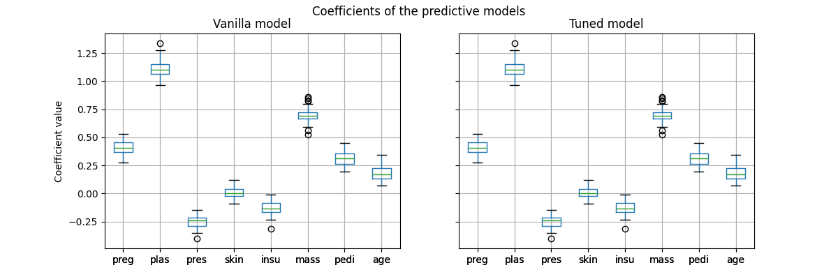
Coefficients of the predictive models, Vanilla model, Tuned model

交叉验证期间仅改变了每个模型的决策阈值。

decision_threshold = pd.Series(
    [est.best_threshold_ for est in cv_results_tuned_model["estimator"]],
)
ax = decision_threshold.plot.kde()
ax.axvline(
    decision_threshold.mean(),
    color="k",
    linestyle="--",
    label=f"Mean decision threshold: {decision_threshold.mean():.2f}",
)
ax.set_xlabel("Decision threshold")
ax.legend(loc="upper right")
_ = ax.set_title(
    "Distribution of the decision threshold \nacross different cross-validation folds"
)

Distribution of the decision threshold across different cross-validation folds

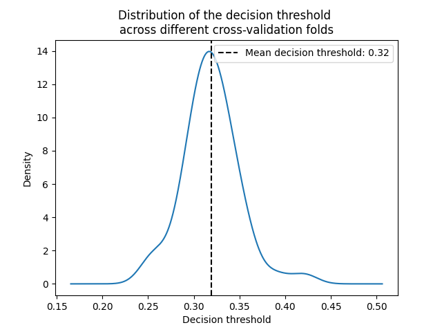
平均而言，0.32左右的决策阈值可以最大化平衡准确性，这与默认决策阈值0.5不同。因此，当使用预测模型的输出来做出决策时，调整决策阈值尤其重要。此外，应仔细选择用于调整决策阈值的指标。在这里，我们使用了平衡的准确性，但它可能不是当前问题的最合适的指标。“正确”指标的选择通常取决于问题，并且可能需要一些领域知识。请参阅标题为， sphx_glr_auto_examples_model_selection_plot_cost_sensitive_learning.py ，了解更多详细信息。

Total running time of the script: （0分29.704秒）