备注
Go to the end 下载完整的示例代码。或者通过浏览器中的MysterLite或Binder运行此示例
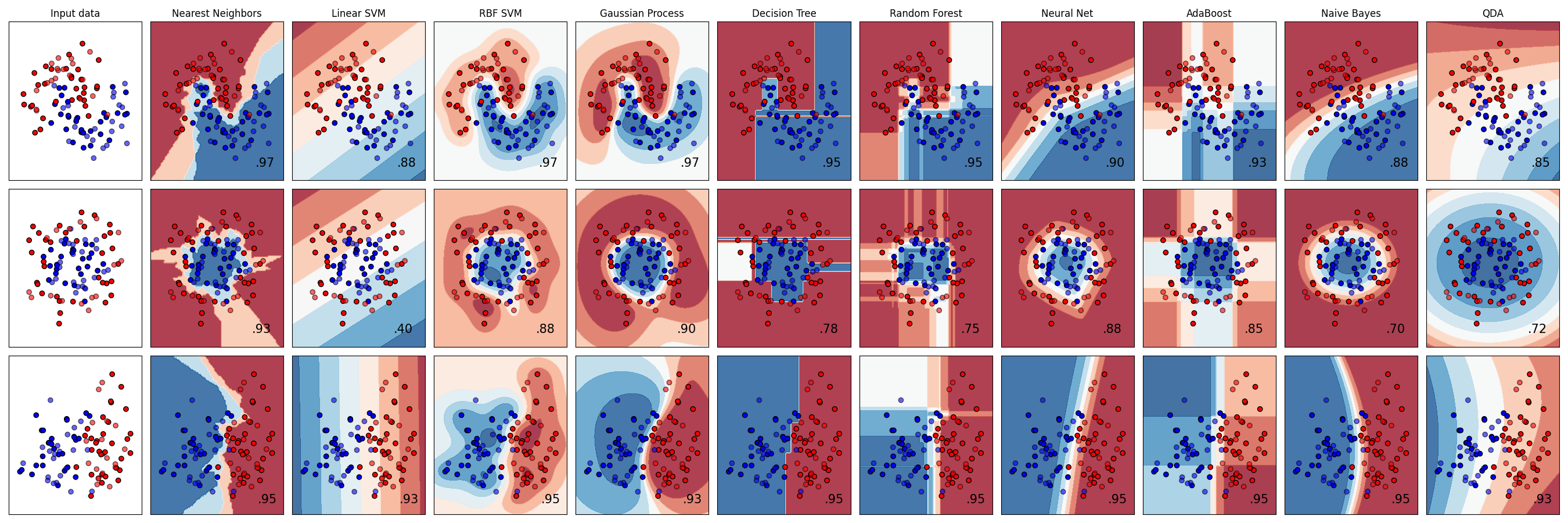
分类器比较#
合成数据集上scikit-learn中的几个分类器的比较。这个例子的重点是说明不同分类器的决策边界的性质。对此应该持保留态度,因为这些例子所传达的直觉不一定会延续到真实的数据集中。
特别是在多维空间中,数据可以更容易地线性分离,而朴素Bayes和线性支持者等分类器的简单性可能会带来比其他分类器更好的概括。
这些图以单色显示训练点,而半透明的测试点。右下角显示测试集的分类准确性。
# Authors: The scikit-learn developers
# SPDX-License-Identifier: BSD-3-Clause

import matplotlib.pyplot as plt
import numpy as np
from matplotlib.colors import ListedColormap

from sklearn.datasets import make_circles, make_classification, make_moons
from sklearn.discriminant_analysis import QuadraticDiscriminantAnalysis
from sklearn.ensemble import AdaBoostClassifier, RandomForestClassifier
from sklearn.gaussian_process import GaussianProcessClassifier
from sklearn.gaussian_process.kernels import RBF
from sklearn.inspection import DecisionBoundaryDisplay
from sklearn.model_selection import train_test_split
from sklearn.naive_bayes import GaussianNB
from sklearn.neighbors import KNeighborsClassifier
from sklearn.neural_network import MLPClassifier
from sklearn.pipeline import make_pipeline
from sklearn.preprocessing import StandardScaler
from sklearn.svm import SVC
from sklearn.tree import DecisionTreeClassifier

names = [
    "Nearest Neighbors",
    "Linear SVM",
    "RBF SVM",
    "Gaussian Process",
    "Decision Tree",
    "Random Forest",
    "Neural Net",
    "AdaBoost",
    "Naive Bayes",
    "QDA",
]

classifiers = [
    KNeighborsClassifier(3),
    SVC(kernel="linear", C=0.025, random_state=42),
    SVC(gamma=2, C=1, random_state=42),
    GaussianProcessClassifier(1.0 * RBF(1.0), random_state=42),
    DecisionTreeClassifier(max_depth=5, random_state=42),
    RandomForestClassifier(
        max_depth=5, n_estimators=10, max_features=1, random_state=42
    ),
    MLPClassifier(alpha=1, max_iter=1000, random_state=42),
    AdaBoostClassifier(random_state=42),
    GaussianNB(),
    QuadraticDiscriminantAnalysis(),
]

X, y = make_classification(
    n_features=2, n_redundant=0, n_informative=2, random_state=1, n_clusters_per_class=1
)
rng = np.random.RandomState(2)
X += 2 * rng.uniform(size=X.shape)
linearly_separable = (X, y)

datasets = [
    make_moons(noise=0.3, random_state=0),
    make_circles(noise=0.2, factor=0.5, random_state=1),
    linearly_separable,
]

figure = plt.figure(figsize=(27, 9))
i = 1
# iterate over datasets
for ds_cnt, ds in enumerate(datasets):
    # preprocess dataset, split into training and test part
    X, y = ds
    X_train, X_test, y_train, y_test = train_test_split(
        X, y, test_size=0.4, random_state=42
    )

    x_min, x_max = X[:, 0].min() - 0.5, X[:, 0].max() + 0.5
    y_min, y_max = X[:, 1].min() - 0.5, X[:, 1].max() + 0.5

    # just plot the dataset first
    cm = plt.cm.RdBu
    cm_bright = ListedColormap(["#FF0000", "#0000FF"])
    ax = plt.subplot(len(datasets), len(classifiers) + 1, i)
    if ds_cnt == 0:
        ax.set_title("Input data")
    # Plot the training points
    ax.scatter(X_train[:, 0], X_train[:, 1], c=y_train, cmap=cm_bright, edgecolors="k")
    # Plot the testing points
    ax.scatter(
        X_test[:, 0], X_test[:, 1], c=y_test, cmap=cm_bright, alpha=0.6, edgecolors="k"
    )
    ax.set_xlim(x_min, x_max)
    ax.set_ylim(y_min, y_max)
    ax.set_xticks(())
    ax.set_yticks(())
    i += 1

    # iterate over classifiers
    for name, clf in zip(names, classifiers):
        ax = plt.subplot(len(datasets), len(classifiers) + 1, i)

        clf = make_pipeline(StandardScaler(), clf)
        clf.fit(X_train, y_train)
        score = clf.score(X_test, y_test)
        DecisionBoundaryDisplay.from_estimator(
            clf, X, cmap=cm, alpha=0.8, ax=ax, eps=0.5
        )

        # Plot the training points
        ax.scatter(
            X_train[:, 0], X_train[:, 1], c=y_train, cmap=cm_bright, edgecolors="k"
        )
        # Plot the testing points
        ax.scatter(
            X_test[:, 0],
            X_test[:, 1],
            c=y_test,
            cmap=cm_bright,
            edgecolors="k",
            alpha=0.6,
        )

        ax.set_xlim(x_min, x_max)
        ax.set_ylim(y_min, y_max)
        ax.set_xticks(())
        ax.set_yticks(())
        if ds_cnt == 0:
            ax.set_title(name)
        ax.text(
            x_max - 0.3,
            y_min + 0.3,
            ("%.2f" % score).lstrip("0"),
            size=15,
            horizontalalignment="right",
        )
        i += 1

plt.tight_layout()
plt.show()
Total running time of the script: (0分1.894秒)
相关实例
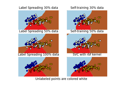
Decision boundary of semi-supervised classifiers versus SVM on the Iris dataset
Gallery generated by Sphinx-Gallery <https://sphinx-gallery.github.io> _