高斯混合模型顺曲线#

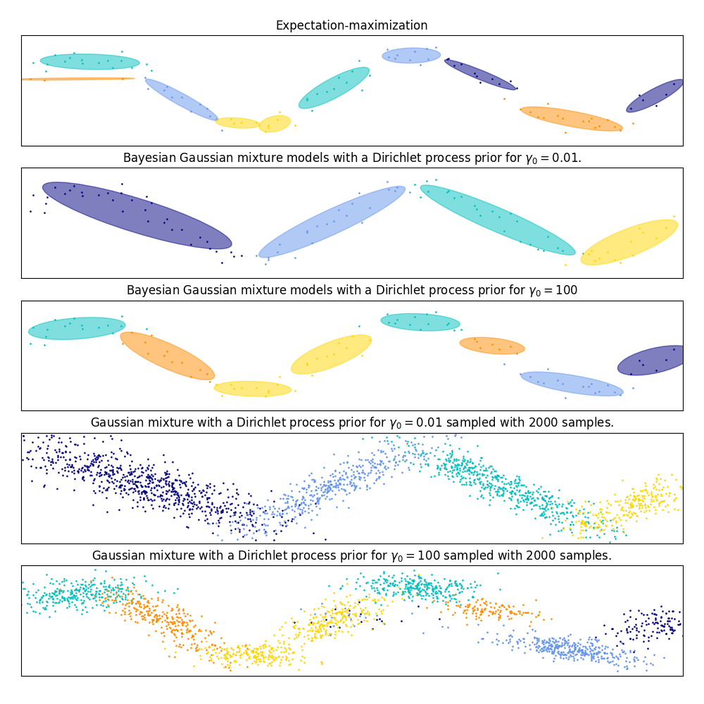
此示例演示了高斯混合模型在不是从高斯随机变量混合中采样的数据上的拟合行为。该数据集由100个点组成，这些点沿着一条嘈杂的正弦曲线松散地分布。因此，对于高斯分量的数量没有地面真值。

第一个模型是经典的高斯混合模型，具有10个分量，符合期望最大化算法。

第二个模型是具有Dirichlet过程先验匹配和变分推理的Bayesian Gaussian混合模型。浓度先验值较低使得模型有利于较少数量的活性成分。该模型“决定”将其建模能力集中在数据集结构的大局上：由非对角协方差矩阵建模的具有交替方向的点组。这些交替方向大致捕捉了原始sin信号的交替性质。

第三个模型也是具有Dirichlet过程先验的Bayesian Gaussian混合模型，但这次浓度先验的值更高，使模型更自由地对数据的细粒度结构进行建模。结果是具有更多活性组件的混合物，这与我们任意决定将组件数量固定为10的第一个模型类似。

哪个模型是最好的是一个主观判断的问题：我们是想要选择只捕捉大局的模型来总结和解释大部分数据结构而忽略细节的模型，还是更喜欢密切关注信号高密度区域的模型？

最后两个面板展示了我们如何从最后两个模型中进行采样。产生的样本分布看起来与原始数据分布并不完全相同。这种差异主要源于我们使用一个模型产生的逼近误差，该模型假设数据是由有限数量的高斯分量而不是连续有噪的sin曲线生成的。

$Expectation-maximization, Bayesian Gaussian mixture models with a Dirichlet process prior for $\gamma_0=0.01$., Gaussian mixture with a Dirichlet process prior for $\gamma_0=0.01$ sampled with $2000$ samples., Bayesian Gaussian mixture models with a Dirichlet process prior for $\gamma_0=100$, Gaussian mixture with a Dirichlet process prior for $\gamma_0=100$ sampled with $2000$ samples.$

# Authors: The scikit-learn developers
# SPDX-License-Identifier: BSD-3-Clause

import itertools

import matplotlib as mpl
import matplotlib.pyplot as plt
import numpy as np
from scipy import linalg

from sklearn import mixture

color_iter = itertools.cycle(["navy", "c", "cornflowerblue", "gold", "darkorange"])


def plot_results(X, Y, means, covariances, index, title):
    splot = plt.subplot(5, 1, 1 + index)
    for i, (mean, covar, color) in enumerate(zip(means, covariances, color_iter)):
        v, w = linalg.eigh(covar)
        v = 2.0 * np.sqrt(2.0) * np.sqrt(v)
        u = w[0] / linalg.norm(w[0])
        # as the DP will not use every component it has access to
        # unless it needs it, we shouldn't plot the redundant
        # components.
        if not np.any(Y == i):
            continue
        plt.scatter(X[Y == i, 0], X[Y == i, 1], 0.8, color=color)

        # Plot an ellipse to show the Gaussian component
        angle = np.arctan(u[1] / u[0])
        angle = 180.0 * angle / np.pi  # convert to degrees
        ell = mpl.patches.Ellipse(mean, v[0], v[1], angle=180.0 + angle, color=color)
        ell.set_clip_box(splot.bbox)
        ell.set_alpha(0.5)
        splot.add_artist(ell)

    plt.xlim(-6.0, 4.0 * np.pi - 6.0)
    plt.ylim(-5.0, 5.0)
    plt.title(title)
    plt.xticks(())
    plt.yticks(())


def plot_samples(X, Y, n_components, index, title):
    plt.subplot(5, 1, 4 + index)
    for i, color in zip(range(n_components), color_iter):
        # as the DP will not use every component it has access to
        # unless it needs it, we shouldn't plot the redundant
        # components.
        if not np.any(Y == i):
            continue
        plt.scatter(X[Y == i, 0], X[Y == i, 1], 0.8, color=color)

    plt.xlim(-6.0, 4.0 * np.pi - 6.0)
    plt.ylim(-5.0, 5.0)
    plt.title(title)
    plt.xticks(())
    plt.yticks(())


# Parameters
n_samples = 100

# Generate random sample following a sine curve
np.random.seed(0)
X = np.zeros((n_samples, 2))
step = 4.0 * np.pi / n_samples

for i in range(X.shape[0]):
    x = i * step - 6.0
    X[i, 0] = x + np.random.normal(0, 0.1)
    X[i, 1] = 3.0 * (np.sin(x) + np.random.normal(0, 0.2))

plt.figure(figsize=(10, 10))
plt.subplots_adjust(
    bottom=0.04, top=0.95, hspace=0.2, wspace=0.05, left=0.03, right=0.97
)

# Fit a Gaussian mixture with EM using ten components
gmm = mixture.GaussianMixture(
    n_components=10, covariance_type="full", max_iter=100
).fit(X)
plot_results(
    X, gmm.predict(X), gmm.means_, gmm.covariances_, 0, "Expectation-maximization"
)

dpgmm = mixture.BayesianGaussianMixture(
    n_components=10,
    covariance_type="full",
    weight_concentration_prior=1e-2,
    weight_concentration_prior_type="dirichlet_process",
    mean_precision_prior=1e-2,
    covariance_prior=1e0 * np.eye(2),
    init_params="random",
    max_iter=100,
    random_state=2,
).fit(X)
plot_results(
    X,
    dpgmm.predict(X),
    dpgmm.means_,
    dpgmm.covariances_,
    1,
    "Bayesian Gaussian mixture models with a Dirichlet process prior "
    r"for $\gamma_0=0.01$.",
)

X_s, y_s = dpgmm.sample(n_samples=2000)
plot_samples(
    X_s,
    y_s,
    dpgmm.n_components,
    0,
    "Gaussian mixture with a Dirichlet process prior "
    r"for $\gamma_0=0.01$ sampled with $2000$ samples.",
)

dpgmm = mixture.BayesianGaussianMixture(
    n_components=10,
    covariance_type="full",
    weight_concentration_prior=1e2,
    weight_concentration_prior_type="dirichlet_process",
    mean_precision_prior=1e-2,
    covariance_prior=1e0 * np.eye(2),
    init_params="kmeans",
    max_iter=100,
    random_state=2,
).fit(X)
plot_results(
    X,
    dpgmm.predict(X),
    dpgmm.means_,
    dpgmm.covariances_,
    2,
    "Bayesian Gaussian mixture models with a Dirichlet process prior "
    r"for $\gamma_0=100$",
)

X_s, y_s = dpgmm.sample(n_samples=2000)
plot_samples(
    X_s,
    y_s,
    dpgmm.n_components,
    1,
    "Gaussian mixture with a Dirichlet process prior "
    r"for $\gamma_0=100$ sampled with $2000$ samples.",
)

plt.show()

Total running time of the script: （0分0.421秒）