备注

Go to the end 下载完整的示例代码。或者通过浏览器中的MysterLite或Binder运行此示例

使用高斯过程回归（GPT）预测Mona Loa数据集的二氧化碳水平#

此示例基于“机器学习的高斯过程”的第5.4.3节 [1]. 它说明了复杂核工程和使用对log边际似然的梯度上升的超参数优化的示例。该数据包括1958年至2001年间夏威夷莫纳罗亚天文台收集的月平均大气二氧化碳浓度（以百万分之一体积（ppm）计）。目标是对CO2浓度作为时间函数进行建模 \(t\) 并推断2001年之后的几年。

引用

print(__doc__)

# Authors: The scikit-learn developers
# SPDX-License-Identifier: BSD-3-Clause

构建数据集#

我们将从莫纳罗亚天文台获取收集空气样本的数据集。我们有兴趣估计二氧化碳的浓度并将其外推至下一年。首先，我们将OpenML中可用的原始数据集作为pandas rame加载。这将被Polars取代一次 fetch_openml 为其添加了本地支持。

from sklearn.datasets import fetch_openml

co2 = fetch_openml(data_id=41187, as_frame=True)
co2.frame.head()

	year	month	day	weight	station	co2
0	1958	3	29	4	MLO	316.1
1	1958	4	5	6	MLO	317.3
2	1958	4	12	4	MLO	317.6
3	1958	4	19	6	MLO	317.5
4	1958	4	26	2	MLO	316.4

首先，我们处理原始的收件箱以创建一个日期列，并将其与CO2列一起选择。

import polars as pl

co2_data = pl.DataFrame(co2.frame[["year", "month", "day", "co2"]]).select(
    pl.date("year", "month", "day"), "co2"
)
co2_data.head()

shape: (5, 2)

date	co2
date	f64
1958-03-29	316.1
1958-04-05	317.3
1958-04-12	317.6
1958-04-19	317.5
1958-04-26	316.4

co2_data["date"].min(), co2_data["date"].max()

(datetime.date(1958, 3, 29), datetime.date(2001, 12, 29))

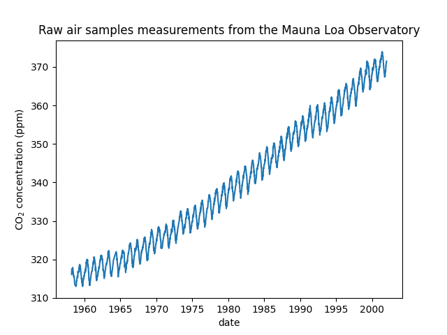
我们看到从1958年3月到2001年12月的某些日子里我们得到了二氧化碳浓度。我们可以绘制这些原始信息以更好地理解。

import matplotlib.pyplot as plt

plt.plot(co2_data["date"], co2_data["co2"])
plt.xlabel("date")
plt.ylabel("CO$_2$ concentration (ppm)")
_ = plt.title("Raw air samples measurements from the Mauna Loa Observatory")

Raw air samples measurements from the Mauna Loa Observatory

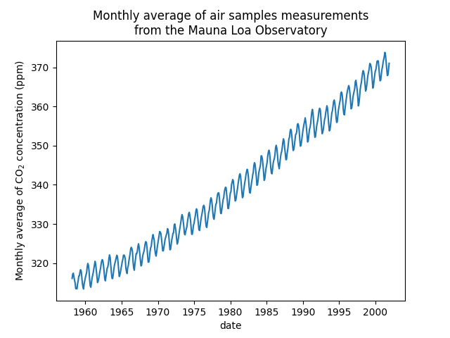
我们将通过获取未收集测量值的月度平均值和下降月份来预处理数据集。这样的处理将对数据产生平滑效果。

co2_data = (
    co2_data.sort(by="date")
    .group_by_dynamic("date", every="1mo")
    .agg(pl.col("co2").mean())
    .drop_nulls()
)
plt.plot(co2_data["date"], co2_data["co2"])
plt.xlabel("date")
plt.ylabel("Monthly average of CO$_2$ concentration (ppm)")
_ = plt.title(
    "Monthly average of air samples measurements\nfrom the Mauna Loa Observatory"
)

Monthly average of air samples measurements from the Mauna Loa Observatory

本例中的想法是预测二氧化碳浓度与日期的函数关系。我们也有兴趣推断2001年之后的来年。

作为第一步，我们将划分数据和目标进行估计。数据是日期，我们将其转换为数字。

X = co2_data.select(
    pl.col("date").dt.year() + pl.col("date").dt.month() / 12
).to_numpy()
y = co2_data["co2"].to_numpy()

设计合适的内核#

为了设计与高斯过程一起使用的内核，我们可以对手头的数据做出一些假设。我们观察到它们有几个特征：我们看到长期上升趋势、明显的季节性变化和一些较小的不规则性。我们可以使用不同的适当内核来捕获这些功能。

首先，可以使用具有大长度尺度参数的辐射基函数（RBS）核来模拟长期上升趋势。具有大长度规模的RBS核强制该分量光滑。没有强制执行趋势性增长，以便为我们的模型提供一定程度的自由度。具体的长度尺度和幅度是免费的超参数。

from sklearn.gaussian_process.kernels import RBF

long_term_trend_kernel = 50.0**2 * RBF(length_scale=50.0)

季节性变化由固定周期为1年的周期性指数sin平方核来解释。控制其平滑度的该周期分量的长度尺度是一个自由参数。为了允许衰变偏离精确的周期性，采用具有RBS核的产品。该RBS组件的长度范围控制衰减时间，并且是另一个自由参数。这种类型的内核也称为局部周期内核。

from sklearn.gaussian_process.kernels import ExpSineSquared

seasonal_kernel = (
    2.0**2
    * RBF(length_scale=100.0)
    * ExpSineSquared(length_scale=1.0, periodicity=1.0, periodicity_bounds="fixed")
)

小的不规则性是由一个合理的二次内核组件，其长度尺度和阿尔法参数，量化的扩散的长度尺度，是要确定的解释。有理二次核等价于具有几个长度尺度的RBF核，并且将更好地适应不同的不规则性。

from sklearn.gaussian_process.kernels import RationalQuadratic

irregularities_kernel = 0.5**2 * RationalQuadratic(length_scale=1.0, alpha=1.0)

最后，数据集中的噪声可以用由RBF核贡献组成的核来解释，这将解释相关的噪声分量，例如局部天气现象，以及白噪声的白核贡献。相对振幅和RBF的长度尺度是另外的自由参数。

from sklearn.gaussian_process.kernels import WhiteKernel

noise_kernel = 0.1**2 * RBF(length_scale=0.1) + WhiteKernel(
    noise_level=0.1**2, noise_level_bounds=(1e-5, 1e5)
)

因此，我们的最终内核是所有之前内核的添加。

co2_kernel = (
    long_term_trend_kernel + seasonal_kernel + irregularities_kernel + noise_kernel
)
co2_kernel

50**2 * RBF(length_scale=50) + 2**2 * RBF(length_scale=100) * ExpSineSquared(length_scale=1, periodicity=1) + 0.5**2 * RationalQuadratic(alpha=1, length_scale=1) + 0.1**2 * RBF(length_scale=0.1) + WhiteKernel(noise_level=0.01)

模型匹配和外推#

现在，我们已经准备好使用高斯过程回归量并适应可用数据了。为了遵循文献中的例子，我们将从目标中减去平均值。我们可以使用 normalize_y=True .然而，这样做也会扩大目标（划分 y 通过其标准差）。因此，不同内核的超参数将具有不同的含义，因为它们不会以ppm表示。

from sklearn.gaussian_process import GaussianProcessRegressor

y_mean = y.mean()
gaussian_process = GaussianProcessRegressor(kernel=co2_kernel, normalize_y=False)
gaussian_process.fit(X, y - y_mean)

GaussianProcessRegressor(kernel=50**2 * RBF(length_scale=50) + 2**2 * RBF(length_scale=100) * ExpSineSquared(length_scale=1, periodicity=1) + 0.5**2 * RationalQuadratic(alpha=1, length_scale=1) + 0.1**2 * RBF(length_scale=0.1) + WhiteKernel(noise_level=0.01))

In a Jupyter environment, please rerun this cell to show the HTML representation or trust the notebook.
On GitHub, the HTML representation is unable to render, please try loading this page with nbviewer.org.

现在，我们将使用高斯过程来预测：

训练数据来检查适合度;
未来的数据来查看模型所做的外推。

因此，我们创建了从1958年到本月的合成数据。此外，我们需要添加训练期间计算的减去平均值。

import datetime

import numpy as np

today = datetime.datetime.now()
current_month = today.year + today.month / 12
X_test = np.linspace(start=1958, stop=current_month, num=1_000).reshape(-1, 1)
mean_y_pred, std_y_pred = gaussian_process.predict(X_test, return_std=True)
mean_y_pred += y_mean

plt.plot(X, y, color="black", linestyle="dashed", label="Measurements")
plt.plot(X_test, mean_y_pred, color="tab:blue", alpha=0.4, label="Gaussian process")
plt.fill_between(
    X_test.ravel(),
    mean_y_pred - std_y_pred,
    mean_y_pred + std_y_pred,
    color="tab:blue",
    alpha=0.2,
)
plt.legend()
plt.xlabel("Year")
plt.ylabel("Monthly average of CO$_2$ concentration (ppm)")
_ = plt.title(
    "Monthly average of air samples measurements\nfrom the Mauna Loa Observatory"
)

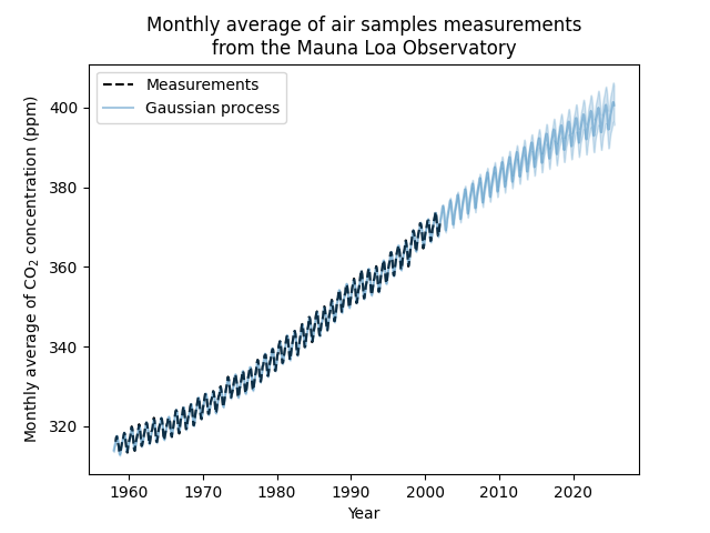
我们的匹配模型能够正确地匹配之前的数据，并自信地外推到未来一年。

核超参数的解释#

现在，我们可以看看内核的超参数。

gaussian_process.kernel_

44.8**2 * RBF(length_scale=51.6) + 2.64**2 * RBF(length_scale=91.5) * ExpSineSquared(length_scale=1.48, periodicity=1) + 0.536**2 * RationalQuadratic(alpha=2.89, length_scale=0.968) + 0.188**2 * RBF(length_scale=0.122) + WhiteKernel(noise_level=0.0367)

因此，减去平均值后，大部分目标信号可以用~45 ppm的长期上升趋势和~52年的长度尺度来解释。周期分量的幅度约为2.6ppm，衰变时间约为90年，长度范围约为1.5。长的衰变时间表明我们有一个非常接近季节周期性的成分。相关噪音的幅度约为0.2 ppm，长度尺度约为0.12年，白噪音贡献约为0.04 ppm。因此，总体噪音水平非常小，这表明该模型可以很好地解释数据。

Total running time of the script: （0分4.994秒）