scikit-learn 0.23的发布亮点

我们很高兴宣布scikit-learn 0.23的发布！添加了许多错误修复和改进，以及一些新的关键功能。我们在下面详细介绍了该版本的一些主要功能。 For an exhaustive list of all the changes ，请参阅 release notes .

安装最新版本（使用pip）：

pip install --upgrade scikit-learn

或带有conda：：

conda install -c conda-forge scikit-learn

广义线性模型和梯度增强的Poisson损失

期待已久的具有非正态损失函数的广义线性模型现已推出。特别是，实施了三个新的回归器： PoissonRegressor , GammaRegressor ，而且 TweedieRegressor . Poisson回归量可用于建模正整数或相对频率。阅读更多的 User Guide .此外， HistGradientBoostingRegressor 也支持新的“poisson”损失。

import numpy as np

from sklearn.ensemble import HistGradientBoostingRegressor
from sklearn.linear_model import PoissonRegressor
from sklearn.model_selection import train_test_split

n_samples, n_features = 1000, 20
rng = np.random.RandomState(0)
X = rng.randn(n_samples, n_features)
# positive integer target correlated with X[:, 5] with many zeros:
y = rng.poisson(lam=np.exp(X[:, 5]) / 2)
X_train, X_test, y_train, y_test = train_test_split(X, y, random_state=rng)
glm = PoissonRegressor()
gbdt = HistGradientBoostingRegressor(loss="poisson", learning_rate=0.01)
glm.fit(X_train, y_train)
gbdt.fit(X_train, y_train)
print(glm.score(X_test, y_test))
print(gbdt.score(X_test, y_test))

0.35776189065725783
0.42425183539869415

估计量的丰富视觉表示

现在，通过启用 display='diagram' 选项.这对于总结管道和其他复合估计器的结构特别有用，并具有交互性以提供详细信息。 单击下面的示例图像以展开Pipeline元素。 看到 可视化复合估计器 了解如何使用此功能。

from sklearn import set_config
from sklearn.compose import make_column_transformer
from sklearn.impute import SimpleImputer
from sklearn.linear_model import LogisticRegression
from sklearn.pipeline import make_pipeline
from sklearn.preprocessing import OneHotEncoder, StandardScaler

set_config(display="diagram")

num_proc = make_pipeline(SimpleImputer(strategy="median"), StandardScaler())

cat_proc = make_pipeline(
    SimpleImputer(strategy="constant", fill_value="missing"),
    OneHotEncoder(handle_unknown="ignore"),
)

preprocessor = make_column_transformer(
    (num_proc, ("feat1", "feat3")), (cat_proc, ("feat0", "feat2"))
)

clf = make_pipeline(preprocessor, LogisticRegression())
clf

Pipeline(steps=[('columntransformer',
                 ColumnTransformer(transformers=[('pipeline-1',
                                                  Pipeline(steps=[('simpleimputer',
                                                                   SimpleImputer(strategy='median')),
                                                                  ('standardscaler',
                                                                   StandardScaler())]),
                                                  ('feat1', 'feat3')),
                                                 ('pipeline-2',
                                                  Pipeline(steps=[('simpleimputer',
                                                                   SimpleImputer(fill_value='missing',
                                                                                 strategy='constant')),
                                                                  ('onehotencoder',
                                                                   OneHotEncoder(handle_unknown='ignore'))]),
                                                  ('feat0', 'feat2'))])),
                ('logisticregression', LogisticRegression())])

In a Jupyter environment, please rerun this cell to show the HTML representation or trust the notebook.
On GitHub, the HTML representation is unable to render, please try loading this page with nbviewer.org.

KMeans的可扩展性和稳定性改进

的 KMeans 估计器完全重新设计，现在它明显更快、更稳定。此外，Elkan算法现在与稀疏矩阵兼容。估计器使用基于BEP的并行性，而不是依赖于jobib，因此 n_jobs 参数不再起作用。有关如何控制线程数的更多详细信息，请参阅我们的 并行性 notes.

import numpy as np
import scipy

from sklearn.cluster import KMeans
from sklearn.datasets import make_blobs
from sklearn.metrics import completeness_score
from sklearn.model_selection import train_test_split

rng = np.random.RandomState(0)
X, y = make_blobs(random_state=rng)
X = scipy.sparse.csr_matrix(X)
X_train, X_test, _, y_test = train_test_split(X, y, random_state=rng)
kmeans = KMeans(n_init="auto").fit(X_train)
print(completeness_score(kmeans.predict(X_test), y_test))

0.6585602198584782

基于柱状图的梯度增强估计器的改进

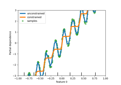
进行了各种改进， HistGradientBoostingClassifier 和 HistGradientBoostingRegressor .在上面提到的泊松损失之上，这些估计量现在支持 sample weights .此外，还增加了自动提前停止条件：样本数量超过10k时默认启用提前停止。最后，用户现在可以定义 monotonic constraints 根据特定特征的变化来约束预测。在下面的例子中，我们构建了一个通常与第一个特征正相关的目标，并带有一些噪音。应用单元约束允许预测捕捉第一个特征的全局效应，而不是适应噪音。有关用例示例，请参阅 梯度增强树的梯度中的功能 .

import numpy as np
from matplotlib import pyplot as plt

from sklearn.ensemble import HistGradientBoostingRegressor

# from sklearn.inspection import plot_partial_dependence
from sklearn.inspection import PartialDependenceDisplay
from sklearn.model_selection import train_test_split

n_samples = 500
rng = np.random.RandomState(0)
X = rng.randn(n_samples, 2)
noise = rng.normal(loc=0.0, scale=0.01, size=n_samples)
y = 5 * X[:, 0] + np.sin(10 * np.pi * X[:, 0]) - noise

gbdt_no_cst = HistGradientBoostingRegressor().fit(X, y)
gbdt_cst = HistGradientBoostingRegressor(monotonic_cst=[1, 0]).fit(X, y)

# plot_partial_dependence has been removed in version 1.2. From 1.2, use
# PartialDependenceDisplay instead.
# disp = plot_partial_dependence(
disp = PartialDependenceDisplay.from_estimator(
    gbdt_no_cst,
    X,
    features=[0],
    feature_names=["feature 0"],
    line_kw={"linewidth": 4, "label": "unconstrained", "color": "tab:blue"},
)
# plot_partial_dependence(
PartialDependenceDisplay.from_estimator(
    gbdt_cst,
    X,
    features=[0],
    line_kw={"linewidth": 4, "label": "constrained", "color": "tab:orange"},
    ax=disp.axes_,
)
disp.axes_[0, 0].plot(
    X[:, 0], y, "o", alpha=0.5, zorder=-1, label="samples", color="tab:green"
)
disp.axes_[0, 0].set_ylim(-3, 3)
disp.axes_[0, 0].set_xlim(-1, 1)
plt.legend()
plt.show()

支持Lasso和ElasticNet的样本权重

两个线性回归量 Lasso 和 ElasticNet 现在支持样本权重。

import numpy as np

from sklearn.datasets import make_regression
from sklearn.linear_model import Lasso
from sklearn.model_selection import train_test_split

n_samples, n_features = 1000, 20
rng = np.random.RandomState(0)
X, y = make_regression(n_samples, n_features, random_state=rng)
sample_weight = rng.rand(n_samples)
X_train, X_test, y_train, y_test, sw_train, sw_test = train_test_split(
    X, y, sample_weight, random_state=rng
)
reg = Lasso()
reg.fit(X_train, y_train, sample_weight=sw_train)
print(reg.score(X_test, y_test, sw_test))

0.999791942438998

相关实例

scikit-learn 1.4的发布亮点

Release Highlights for scikit-learn 1.4

scikit-learn 0.24发布亮点

Release Highlights for scikit-learn 0.24

单调约束

Monotonic Constraints

scikit-learn 1.0的发布亮点

Release Highlights for scikit-learn 1.0