模型复杂性影响#

演示模型复杂性如何影响预测准确性和计算性能。

我们将使用两个数据集：

糖尿病数据集用于回归。该数据集由从糖尿病患者中获取的10项测量结果组成。任务是预测疾病进展;
20个新闻组文本数据集用于分类。此数据集由新闻组帖子组成。任务是预测该帖子所写的主题（20个主题中）。

我们将对三个不同估计量的复杂性影响进行建模：

SGDClassifier (for分类数据），其实现随机梯度下降学习;
NuSVR (for回归数据），实现Nu支持量回归;
GradientBoostingRegressor 以向前阶段的方式构建添加剂模型。注意到 HistGradientBoostingRegressor 远快于 GradientBoostingRegressor 从中间数据集开始 (n_samples >= 10_000 ），而这个例子的情况并非如此。

我们通过选择每个所选模型中的相关模型参数来使模型复杂性有所不同。接下来，我们将衡量对计算性能（延迟）和预测能力（SSE或海明损失）的影响。

# Authors: The scikit-learn developers
# SPDX-License-Identifier: BSD-3-Clause

import time

import matplotlib.pyplot as plt
import numpy as np

from sklearn import datasets
from sklearn.ensemble import GradientBoostingRegressor
from sklearn.linear_model import SGDClassifier
from sklearn.metrics import hamming_loss, mean_squared_error
from sklearn.model_selection import train_test_split
from sklearn.svm import NuSVR

# Initialize random generator
np.random.seed(0)

加载数据#

首先我们加载这两个数据集。

备注

我们正在使用 fetch_20newsgroups_vectorized 下载20个新闻组数据集。它返回即可使用的功能。

备注

X 20个新闻组数据集是一个稀疏矩阵， X 糖尿病数据集的数据是一个麻木的数组。

def generate_data(case):
    """Generate regression/classification data."""
    if case == "regression":
        X, y = datasets.load_diabetes(return_X_y=True)
        train_size = 0.8
    elif case == "classification":
        X, y = datasets.fetch_20newsgroups_vectorized(subset="all", return_X_y=True)
        train_size = 0.4  # to make the example run faster

    X_train, X_test, y_train, y_test = train_test_split(
        X, y, train_size=train_size, random_state=0
    )

    data = {"X_train": X_train, "X_test": X_test, "y_train": y_train, "y_test": y_test}
    return data


regression_data = generate_data("regression")
classification_data = generate_data("classification")

基准影响力#

接下来，我们可以计算参数对给定估计量的影响。在每一轮中，我们将使用新值来设置估计器 changing_param 我们将收集预测时间、预测性能和复杂性，以了解这些变化如何影响估计器。我们将计算复杂度， complexity_computer 作为参数传递。

def benchmark_influence(conf):
    """
    Benchmark influence of `changing_param` on both MSE and latency.
    """
    prediction_times = []
    prediction_powers = []
    complexities = []
    for param_value in conf["changing_param_values"]:
        conf["tuned_params"][conf["changing_param"]] = param_value
        estimator = conf["estimator"](**conf["tuned_params"])

        print("Benchmarking %s" % estimator)
        estimator.fit(conf["data"]["X_train"], conf["data"]["y_train"])
        conf["postfit_hook"](estimator)
        complexity = conf["complexity_computer"](estimator)
        complexities.append(complexity)
        start_time = time.time()
        for _ in range(conf["n_samples"]):
            y_pred = estimator.predict(conf["data"]["X_test"])
        elapsed_time = (time.time() - start_time) / float(conf["n_samples"])
        prediction_times.append(elapsed_time)
        pred_score = conf["prediction_performance_computer"](
            conf["data"]["y_test"], y_pred
        )
        prediction_powers.append(pred_score)
        print(
            "Complexity: %d | %s: %.4f | Pred. Time: %fs\n"
            % (
                complexity,
                conf["prediction_performance_label"],
                pred_score,
                elapsed_time,
            )
        )
    return prediction_powers, prediction_times, complexities

选择参数#

我们通过制作包含所有必要值的字典来选择每个估计器的参数。 changing_param 是参数的名称，该参数在每个估计器中都会有所不同。复杂性将由 complexity_label 并计算使用 complexity_computer .另请注意，根据估计器类型，我们传递不同的数据。

def _count_nonzero_coefficients(estimator):
    a = estimator.coef_.toarray()
    return np.count_nonzero(a)


configurations = [
    {
        "estimator": SGDClassifier,
        "tuned_params": {
            "penalty": "elasticnet",
            "alpha": 0.001,
            "loss": "modified_huber",
            "fit_intercept": True,
            "tol": 1e-1,
            "n_iter_no_change": 2,
        },
        "changing_param": "l1_ratio",
        "changing_param_values": [0.25, 0.5, 0.75, 0.9],
        "complexity_label": "non_zero coefficients",
        "complexity_computer": _count_nonzero_coefficients,
        "prediction_performance_computer": hamming_loss,
        "prediction_performance_label": "Hamming Loss (Misclassification Ratio)",
        "postfit_hook": lambda x: x.sparsify(),
        "data": classification_data,
        "n_samples": 5,
    },
    {
        "estimator": NuSVR,
        "tuned_params": {"C": 1e3, "gamma": 2**-15},
        "changing_param": "nu",
        "changing_param_values": [0.05, 0.1, 0.2, 0.35, 0.5],
        "complexity_label": "n_support_vectors",
        "complexity_computer": lambda x: len(x.support_vectors_),
        "data": regression_data,
        "postfit_hook": lambda x: x,
        "prediction_performance_computer": mean_squared_error,
        "prediction_performance_label": "MSE",
        "n_samples": 15,
    },
    {
        "estimator": GradientBoostingRegressor,
        "tuned_params": {
            "loss": "squared_error",
            "learning_rate": 0.05,
            "max_depth": 2,
        },
        "changing_param": "n_estimators",
        "changing_param_values": [10, 25, 50, 75, 100],
        "complexity_label": "n_trees",
        "complexity_computer": lambda x: x.n_estimators,
        "data": regression_data,
        "postfit_hook": lambda x: x,
        "prediction_performance_computer": mean_squared_error,
        "prediction_performance_label": "MSE",
        "n_samples": 15,
    },
]

Run the code and plot the results#

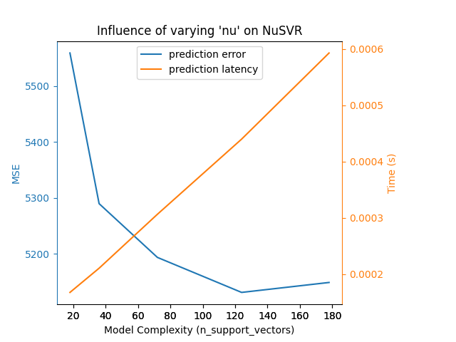
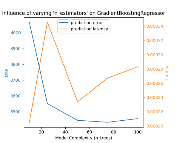
我们定义了运行基准所需的所有功能。现在，我们将循环讨论之前定义的不同配置。随后，我们可以分析从基准中获得的地块：放松 L1 BCD分类器中的惩罚减少了预测误差，但导致训练时间增加。我们可以对训练时间进行类似的分析，训练时间随着Nu-SVR的支持载体数量的增加而增加。然而，我们观察到存在最佳数量的支持载体可以减少预测误差。事实上，支持载体太少会导致模型不充分，而支持载体太多会导致模型不充分。对于梯度提升模型可以得出完全相同的结论。与Nu-SVR的唯一区别是，整体中有太多的树并没有那么有害。

def plot_influence(conf, mse_values, prediction_times, complexities):
    """
    Plot influence of model complexity on both accuracy and latency.
    """

    fig = plt.figure()
    fig.subplots_adjust(right=0.75)

    # first axes (prediction error)
    ax1 = fig.add_subplot(111)
    line1 = ax1.plot(complexities, mse_values, c="tab:blue", ls="-")[0]
    ax1.set_xlabel("Model Complexity (%s)" % conf["complexity_label"])
    y1_label = conf["prediction_performance_label"]
    ax1.set_ylabel(y1_label)

    ax1.spines["left"].set_color(line1.get_color())
    ax1.yaxis.label.set_color(line1.get_color())
    ax1.tick_params(axis="y", colors=line1.get_color())

    # second axes (latency)
    ax2 = fig.add_subplot(111, sharex=ax1, frameon=False)
    line2 = ax2.plot(complexities, prediction_times, c="tab:orange", ls="-")[0]
    ax2.yaxis.tick_right()
    ax2.yaxis.set_label_position("right")
    y2_label = "Time (s)"
    ax2.set_ylabel(y2_label)
    ax1.spines["right"].set_color(line2.get_color())
    ax2.yaxis.label.set_color(line2.get_color())
    ax2.tick_params(axis="y", colors=line2.get_color())

    plt.legend(
        (line1, line2), ("prediction error", "prediction latency"), loc="upper center"
    )

    plt.title(
        "Influence of varying '%s' on %s"
        % (conf["changing_param"], conf["estimator"].__name__)
    )


for conf in configurations:
    prediction_performances, prediction_times, complexities = benchmark_influence(conf)
    plot_influence(conf, prediction_performances, prediction_times, complexities)
plt.show()

Benchmarking SGDClassifier(alpha=0.001, l1_ratio=0.25, loss='modified_huber',
              n_iter_no_change=2, penalty='elasticnet', tol=0.1)
Complexity: 4948 | Hamming Loss (Misclassification Ratio): 0.2675 | Pred. Time: 0.060023s

Benchmarking SGDClassifier(alpha=0.001, l1_ratio=0.5, loss='modified_huber',
              n_iter_no_change=2, penalty='elasticnet', tol=0.1)
Complexity: 1847 | Hamming Loss (Misclassification Ratio): 0.3264 | Pred. Time: 0.043359s

Benchmarking SGDClassifier(alpha=0.001, l1_ratio=0.75, loss='modified_huber',
              n_iter_no_change=2, penalty='elasticnet', tol=0.1)
Complexity: 997 | Hamming Loss (Misclassification Ratio): 0.3383 | Pred. Time: 0.036040s

Benchmarking SGDClassifier(alpha=0.001, l1_ratio=0.9, loss='modified_huber',
              n_iter_no_change=2, penalty='elasticnet', tol=0.1)
Complexity: 802 | Hamming Loss (Misclassification Ratio): 0.3582 | Pred. Time: 0.032510s

Benchmarking NuSVR(C=1000.0, gamma=3.0517578125e-05, nu=0.05)
Complexity: 18 | MSE: 5558.7313 | Pred. Time: 0.000167s

Benchmarking NuSVR(C=1000.0, gamma=3.0517578125e-05, nu=0.1)
Complexity: 36 | MSE: 5289.8022 | Pred. Time: 0.000210s

Benchmarking NuSVR(C=1000.0, gamma=3.0517578125e-05, nu=0.2)
Complexity: 72 | MSE: 5193.8353 | Pred. Time: 0.000306s

Benchmarking NuSVR(C=1000.0, gamma=3.0517578125e-05, nu=0.35)
Complexity: 124 | MSE: 5131.3279 | Pred. Time: 0.000440s

Benchmarking NuSVR(C=1000.0, gamma=3.0517578125e-05)
Complexity: 178 | MSE: 5149.0779 | Pred. Time: 0.000593s

Benchmarking GradientBoostingRegressor(learning_rate=0.05, max_depth=2, n_estimators=10)
Complexity: 10 | MSE: 4066.4812 | Pred. Time: 0.000205s

Benchmarking GradientBoostingRegressor(learning_rate=0.05, max_depth=2, n_estimators=25)
Complexity: 25 | MSE: 3551.1723 | Pred. Time: 0.000346s

Benchmarking GradientBoostingRegressor(learning_rate=0.05, max_depth=2, n_estimators=50)
Complexity: 50 | MSE: 3445.2171 | Pred. Time: 0.000234s

Benchmarking GradientBoostingRegressor(learning_rate=0.05, max_depth=2, n_estimators=75)
Complexity: 75 | MSE: 3433.0358 | Pred. Time: 0.000267s

Benchmarking GradientBoostingRegressor(learning_rate=0.05, max_depth=2)
Complexity: 100 | MSE: 3456.0602 | Pred. Time: 0.000283s

结论#

作为结论，我们可以推断出以下见解：

更复杂（或表现力）的模型将需要更长的训练时间;
更复杂的模型并不能保证减少预测误差。

这些方面与模型泛化和避免模型欠拟合或过拟合有关。

Total running time of the script: （0分4.662秒）