备注
Go to the end 下载完整的示例代码。或者通过浏览器中的MysterLite或Binder运行此示例
特征缩放的重要性#
通过标准化进行特征缩放(也称为Z得分规范化)是许多机器学习算法的重要预处理步骤。它涉及重新缩放每个特征,使其标准差为1,平均值为0。
即使基于树的模型(几乎)不受缩放的影响,许多其他算法也需要对特征进行规格化,通常出于不同的原因:为了简化收敛(例如无惩罚的逻辑回归),创建与未缩放数据的匹配(例如KNeighbors模型)相比完全不同的模型匹配。后者在本示例的第一部分中得到了演示。
在示例的第二部分,我们展示了特征规范化如何影响主成分分析(PCA)。为了说明这一点,我们比较了使用 PCA 使用未缩放的数据和使用 StandardScaler 首先扩展数据。
在示例的最后一部分中,我们展示了规范化对在PCA精简数据上训练的模型准确性的影响。
# Authors: The scikit-learn developers
# SPDX-License-Identifier: BSD-3-Clause
加载和准备数据#
使用的数据集是 葡萄酒识别数据集 在UCI提供。该数据集具有连续特征,由于测量的属性不同(例如酒精含量和苹果酸),这些特征在规模上是不均匀的。
from sklearn.datasets import load_wine
from sklearn.model_selection import train_test_split
from sklearn.preprocessing import StandardScaler

X, y = load_wine(return_X_y=True, as_frame=True)
scaler = StandardScaler().set_output(transform="pandas")

X_train, X_test, y_train, y_test = train_test_split(
    X, y, test_size=0.30, random_state=42
)
scaled_X_train = scaler.fit_transform(X_train)
重新缩放对k近邻模型的影响#
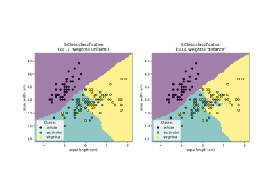
为了可视化的决策边界 KNeighborsClassifier ,在本节中,我们选择具有不同数量级值的2个特征的子集。
请记住,使用特征的子集来训练模型可能会遗漏具有高预测影响的特征,从而导致决策边界比在完整特征集上训练的模型更差。
import matplotlib.pyplot as plt

from sklearn.inspection import DecisionBoundaryDisplay
from sklearn.neighbors import KNeighborsClassifier

X_plot = X[["proline", "hue"]]
X_plot_scaled = scaler.fit_transform(X_plot)
clf = KNeighborsClassifier(n_neighbors=20)


def fit_and_plot_model(X_plot, y, clf, ax):
    clf.fit(X_plot, y)
    disp = DecisionBoundaryDisplay.from_estimator(
        clf,
        X_plot,
        response_method="predict",
        alpha=0.5,
        ax=ax,
    )
    disp.ax_.scatter(X_plot["proline"], X_plot["hue"], c=y, s=20, edgecolor="k")
    disp.ax_.set_xlim((X_plot["proline"].min(), X_plot["proline"].max()))
    disp.ax_.set_ylim((X_plot["hue"].min(), X_plot["hue"].max()))
    return disp.ax_


fig, (ax1, ax2) = plt.subplots(ncols=2, figsize=(12, 6))

fit_and_plot_model(X_plot, y, clf, ax1)
ax1.set_title("KNN without scaling")

fit_and_plot_model(X_plot_scaled, y, clf, ax2)
ax2.set_xlabel("scaled proline")
ax2.set_ylabel("scaled hue")
_ = ax2.set_title("KNN with scaling")

这里的决策边界表明,对缩放或非缩放数据进行匹配会导致完全不同的模型。原因是变量“Pro”的值在0和1,000之间变化;而变量“hue”的值在1和10之间变化。因此,样本之间的距离主要受到“Pro”值差异的影响,而“色调”的值相对会被忽视。如果使用 StandardScaler 为了规范化该数据库,两个缩放值大约在-3和3之间,并且邻居结构将或多或少地受到两个变量的影响。
重新缩放对PCA降维的影响#
使用缩小尺寸 PCA 包括找到使方差最大化的特征。如果一个要素仅因为各自的规模而比其他要素变化更大, PCA 将确定这种特征主导主成分的方向。
我们可以使用所有原始特征检查第一主成分:
import pandas as pd

from sklearn.decomposition import PCA

pca = PCA(n_components=2).fit(X_train)
scaled_pca = PCA(n_components=2).fit(scaled_X_train)
X_train_transformed = pca.transform(X_train)
X_train_std_transformed = scaled_pca.transform(scaled_X_train)

first_pca_component = pd.DataFrame(
    pca.components_[0], index=X.columns, columns=["without scaling"]
)
first_pca_component["with scaling"] = scaled_pca.components_[0]
first_pca_component.plot.bar(
    title="Weights of the first principal component", figsize=(6, 8)
)

_ = plt.tight_layout()
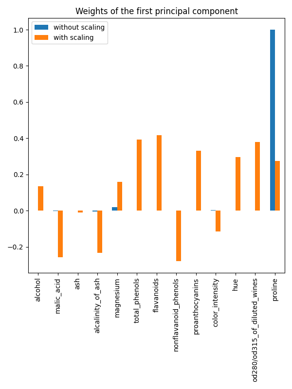
Indeed we find that the "proline" feature dominates the direction of the first principal component without scaling, being about two orders of magnitude above the other features. This is contrasted when observing the first principal component for the scaled version of the data, where the orders of magnitude are roughly the same across all the features.
我们可以可视化这两种情况下主成分的分布:
fig, (ax1, ax2) = plt.subplots(nrows=1, ncols=2, figsize=(10, 5))

target_classes = range(0, 3)
colors = ("blue", "red", "green")
markers = ("^", "s", "o")

for target_class, color, marker in zip(target_classes, colors, markers):
    ax1.scatter(
        x=X_train_transformed[y_train == target_class, 0],
        y=X_train_transformed[y_train == target_class, 1],
        color=color,
        label=f"class {target_class}",
        alpha=0.5,
        marker=marker,
    )

    ax2.scatter(
        x=X_train_std_transformed[y_train == target_class, 0],
        y=X_train_std_transformed[y_train == target_class, 1],
        color=color,
        label=f"class {target_class}",
        alpha=0.5,
        marker=marker,
    )

ax1.set_title("Unscaled training dataset after PCA")
ax2.set_title("Standardized training dataset after PCA")

for ax in (ax1, ax2):
    ax.set_xlabel("1st principal component")
    ax.set_ylabel("2nd principal component")
    ax.legend(loc="upper right")
    ax.grid()

_ = plt.tight_layout()
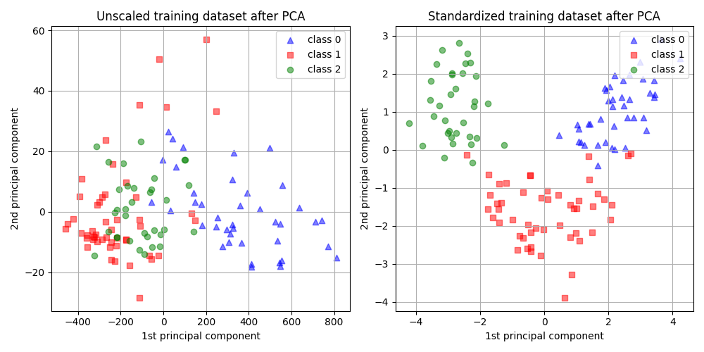
从上面的图中我们观察到,在降低维度之前缩放特征会导致组件具有相同数量级。在这种情况下,它还提高了类的可分离性。事实上,在下一节中,我们确认更好的可分离性对整体模型的性能有良好的影响。
重标度对模型性能的影响#
首先,我们展示如何对一个的最佳正规化 LogisticRegressionCV 取决于数据的扩展或非扩展:
import numpy as np

from sklearn.linear_model import LogisticRegressionCV
from sklearn.pipeline import make_pipeline

Cs = np.logspace(-5, 5, 20)

unscaled_clf = make_pipeline(pca, LogisticRegressionCV(Cs=Cs))
unscaled_clf.fit(X_train, y_train)

scaled_clf = make_pipeline(scaler, pca, LogisticRegressionCV(Cs=Cs))
scaled_clf.fit(X_train, y_train)

print(f"Optimal C for the unscaled PCA: {unscaled_clf[-1].C_[0]:.4f}\n")
print(f"Optimal C for the standardized data with PCA: {scaled_clf[-1].C_[0]:.2f}")
Optimal C for the unscaled PCA: 0.0004

Optimal C for the standardized data with PCA: 20.69
对正规化的需求更高(较低的值 C )对于在应用PCA之前未缩放的数据。我们现在评估缩放对最佳模型的准确性和平均对数损失的影响:
from sklearn.metrics import accuracy_score, log_loss

y_pred = unscaled_clf.predict(X_test)
y_pred_scaled = scaled_clf.predict(X_test)
y_proba = unscaled_clf.predict_proba(X_test)
y_proba_scaled = scaled_clf.predict_proba(X_test)

print("Test accuracy for the unscaled PCA")
print(f"{accuracy_score(y_test, y_pred):.2%}\n")
print("Test accuracy for the standardized data with PCA")
print(f"{accuracy_score(y_test, y_pred_scaled):.2%}\n")
print("Log-loss for the unscaled PCA")
print(f"{log_loss(y_test, y_proba):.3}\n")
print("Log-loss for the standardized data with PCA")
print(f"{log_loss(y_test, y_proba_scaled):.3}")
Test accuracy for the unscaled PCA
35.19%

Test accuracy for the standardized data with PCA
96.30%

Log-loss for the unscaled PCA
0.957

Log-loss for the standardized data with PCA
0.0825
当之前缩放数据时,可以观察到预测准确性的明显差异 PCA ,因为它的性能大大优于未缩放版本。这与从上一节中的图中获得的直觉相对应,其中在使用之前进行缩放时,组件变得线性可分离 PCA .
注意,在这种情况下,具有缩放特征的模型比具有非缩放特征的模型表现得更好,因为所有变量都是预测性的,我们宁愿避免其中一些被相对忽略。
如果较低尺度中的变量不具有预测性,那么缩放特征后可能会出现性能下降:有噪的特征将对缩放后的预测做出更大贡献,因此缩放会增加过度匹配。
最后但并非最不重要的是,我们观察到通过缩放步骤实现了较低的对数损失。
Total running time of the script: (0分1.413秒)
相关实例
Gallery generated by Sphinx-Gallery <https://sphinx-gallery.github.io> _