平衡模型复杂性和交叉验证分数

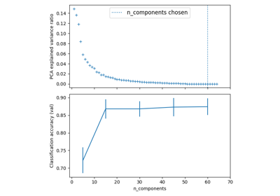
此示例演示了如何平衡模型复杂性和交叉验证分数，方法是在最佳准确性分数的1个标准差内找到不错的准确性，同时最大限度地减少 PCA 组件 [1] .它使用 GridSearchCV 具有可调用的自定义改装以选择最佳型号。

该图显示了交叉验证分数和PCA组件数量之间的权衡。平衡的情况是， n_components=10 和 accuracy=0.88 ，其落入最佳准确度得分1个标准差以内的范围内。

[1] 哈斯蒂，T.，蒂布希拉尼，R.，，Friedman，J.（2001）。模型评估和选择。统计学习的要素（pp。219-260）。美国纽约州纽约：Springer New York Inc..

# Authors: The scikit-learn developers
# SPDX-License-Identifier: BSD-3-Clause

import matplotlib.pyplot as plt
import numpy as np
import polars as pl

from sklearn.datasets import load_digits
from sklearn.decomposition import PCA
from sklearn.linear_model import LogisticRegression
from sklearn.model_selection import GridSearchCV, ShuffleSplit
from sklearn.pipeline import Pipeline

介绍

在调整超参数时，我们通常希望平衡模型复杂性和性能。“一个标准误差”规则是一种常见的方法：选择最简单的模型，其性能在最佳模型性能的一个标准误差内。这有助于避免过度拟合，因为当更简单的模型的性能在统计上与更复杂的模型相当时，更喜欢它们。

辅助功能

我们定义了两个助手函数：1. lower_bound ：计算可接受性能的阈值（最佳得分- 1 std）2. best_low_complexity ：初始化具有超过此阈值的最少PCA组件的模型

def lower_bound(cv_results):
    """
    Calculate the lower bound within 1 standard deviation
    of the best `mean_test_scores`.

    Parameters
    ----------
    cv_results : dict of numpy(masked) ndarrays
        See attribute cv_results_ of `GridSearchCV`

    Returns
    -------
    float
        Lower bound within 1 standard deviation of the
        best `mean_test_score`.
    """
    best_score_idx = np.argmax(cv_results["mean_test_score"])

    return (
        cv_results["mean_test_score"][best_score_idx]
        - cv_results["std_test_score"][best_score_idx]
    )


def best_low_complexity(cv_results):
    """
    Balance model complexity with cross-validated score.

    Parameters
    ----------
    cv_results : dict of numpy(masked) ndarrays
        See attribute cv_results_ of `GridSearchCV`.

    Return
    ------
    int
        Index of a model that has the fewest PCA components
        while has its test score within 1 standard deviation of the best
        `mean_test_score`.
    """
    threshold = lower_bound(cv_results)
    candidate_idx = np.flatnonzero(cv_results["mean_test_score"] >= threshold)
    best_idx = candidate_idx[
        cv_results["param_reduce_dim__n_components"][candidate_idx].argmin()
    ]
    return best_idx

设置管道和参数网格

我们通过两个步骤创建管道：1.使用PCA 2降低主观性。使用LogisticRegulation进行分类

我们将搜索不同数量的PCA组件以找到最佳复杂性。

pipe = Pipeline(
    [
        ("reduce_dim", PCA(random_state=42)),
        ("classify", LogisticRegression(random_state=42, C=0.01, max_iter=1000)),
    ]
)

param_grid = {"reduce_dim__n_components": [6, 8, 10, 15, 20, 25, 35, 45, 55]}

使用GridSearchCV执行搜索

我们使用 GridSearchCV 与我们的习俗 best_low_complexity 用作改装参数。此功能将选择PCA分量最少的模型，该模型的性能仍在最佳模型的一个标准差内。

grid = GridSearchCV(
    pipe,
    # Use a non-stratified CV strategy to make sure that the inter-fold
    # standard deviation of the test scores is informative.
    cv=ShuffleSplit(n_splits=30, random_state=0),
    n_jobs=1,  # increase this on your machine to use more physical cores
    param_grid=param_grid,
    scoring="accuracy",
    refit=best_low_complexity,
    return_train_score=True,
)

加载数字数据集并匹配模型

X, y = load_digits(return_X_y=True)
grid.fit(X, y)

GridSearchCV(cv=ShuffleSplit(n_splits=30, random_state=0, test_size=None, train_size=None),
             estimator=Pipeline(steps=[('reduce_dim', PCA(random_state=42)),
                                       ('classify',
                                        LogisticRegression(C=0.01,
                                                           max_iter=1000,
                                                           random_state=42))]),
             n_jobs=1,
             param_grid={'reduce_dim__n_components': [6, 8, 10, 15, 20, 25, 35,
                                                      45, 55]},
             refit=<function best_low_complexity at 0x7fa26e03c0e0>,
             return_train_score=True, scoring='accuracy')

In a Jupyter environment, please rerun this cell to show the HTML representation or trust the notebook.
On GitHub, the HTML representation is unable to render, please try loading this page with nbviewer.org.

使结果可视化

我们将创建一个条形图，显示不同数量的PCA组件的测试分数，以及指示最佳分数和一个标准差阈值的水平线。

n_components = grid.cv_results_["param_reduce_dim__n_components"]
test_scores = grid.cv_results_["mean_test_score"]

# Create a polars DataFrame for better data manipulation and visualization
results_df = pl.DataFrame(
    {
        "n_components": n_components,
        "mean_test_score": test_scores,
        "std_test_score": grid.cv_results_["std_test_score"],
        "mean_train_score": grid.cv_results_["mean_train_score"],
        "std_train_score": grid.cv_results_["std_train_score"],
        "mean_fit_time": grid.cv_results_["mean_fit_time"],
        "rank_test_score": grid.cv_results_["rank_test_score"],
    }
)

# Sort by number of components
results_df = results_df.sort("n_components")

# Calculate the lower bound threshold
lower = lower_bound(grid.cv_results_)

# Get the best model information
best_index_ = grid.best_index_
best_components = n_components[best_index_]
best_score = grid.cv_results_["mean_test_score"][best_index_]

# Add a column to mark the selected model
results_df = results_df.with_columns(
    pl.when(pl.col("n_components") == best_components)
    .then(pl.lit("Selected"))
    .otherwise(pl.lit("Regular"))
    .alias("model_type")
)

# Get the number of CV splits from the results
n_splits = sum(
    1
    for key in grid.cv_results_.keys()
    if key.startswith("split") and key.endswith("test_score")
)

# Extract individual scores for each split
test_scores = np.array(
    [
        [grid.cv_results_[f"split{i}_test_score"][j] for i in range(n_splits)]
        for j in range(len(n_components))
    ]
)
train_scores = np.array(
    [
        [grid.cv_results_[f"split{i}_train_score"][j] for i in range(n_splits)]
        for j in range(len(n_components))
    ]
)

# Calculate mean and std of test scores
mean_test_scores = np.mean(test_scores, axis=1)
std_test_scores = np.std(test_scores, axis=1)

# Find best score and threshold
best_mean_score = np.max(mean_test_scores)
threshold = best_mean_score - std_test_scores[np.argmax(mean_test_scores)]

# Create a single figure for visualization
fig, ax = plt.subplots(figsize=(12, 8))

# Plot individual points
for i, comp in enumerate(n_components):
    # Plot individual test points
    plt.scatter(
        [comp] * n_splits,
        test_scores[i],
        alpha=0.2,
        color="blue",
        s=20,
        label="Individual test scores" if i == 0 else "",
    )
    # Plot individual train points
    plt.scatter(
        [comp] * n_splits,
        train_scores[i],
        alpha=0.2,
        color="green",
        s=20,
        label="Individual train scores" if i == 0 else "",
    )

# Plot mean lines with error bands
plt.plot(
    n_components,
    np.mean(test_scores, axis=1),
    "-",
    color="blue",
    linewidth=2,
    label="Mean test score",
)
plt.fill_between(
    n_components,
    np.mean(test_scores, axis=1) - np.std(test_scores, axis=1),
    np.mean(test_scores, axis=1) + np.std(test_scores, axis=1),
    alpha=0.15,
    color="blue",
)

plt.plot(
    n_components,
    np.mean(train_scores, axis=1),
    "-",
    color="green",
    linewidth=2,
    label="Mean train score",
)
plt.fill_between(
    n_components,
    np.mean(train_scores, axis=1) - np.std(train_scores, axis=1),
    np.mean(train_scores, axis=1) + np.std(train_scores, axis=1),
    alpha=0.15,
    color="green",
)

# Add threshold lines
plt.axhline(
    best_mean_score,
    color="#9b59b6",  # Purple
    linestyle="--",
    label="Best score",
    linewidth=2,
)
plt.axhline(
    threshold,
    color="#e67e22",  # Orange
    linestyle="--",
    label="Best score - 1 std",
    linewidth=2,
)

# Highlight selected model
plt.axvline(
    best_components,
    color="#9b59b6",  # Purple
    alpha=0.2,
    linewidth=8,
    label="Selected model",
)

# Set titles and labels
plt.xlabel("Number of PCA components", fontsize=12)
plt.ylabel("Score", fontsize=12)
plt.title("Model Selection: Balancing Complexity and Performance", fontsize=14)
plt.grid(True, linestyle="--", alpha=0.7)
plt.legend(
    bbox_to_anchor=(1.02, 1),
    loc="upper left",
    borderaxespad=0,
)

# Set axis properties
plt.xticks(n_components)
plt.ylim((0.85, 1.0))

# # Adjust layout
plt.tight_layout()

打印结果

我们打印有关所选型号的信息，包括其复杂性和性能。我们还显示了使用两极的所有模型的汇总表。

print("Best model selected by the one-standard-error rule:")
print(f"Number of PCA components: {best_components}")
print(f"Accuracy score: {best_score:.4f}")
print(f"Best possible accuracy: {np.max(test_scores):.4f}")
print(f"Accuracy threshold (best - 1 std): {lower:.4f}")

# Create a summary table with polars
summary_df = results_df.select(
    pl.col("n_components"),
    pl.col("mean_test_score").round(4).alias("test_score"),
    pl.col("std_test_score").round(4).alias("test_std"),
    pl.col("mean_train_score").round(4).alias("train_score"),
    pl.col("std_train_score").round(4).alias("train_std"),
    pl.col("mean_fit_time").round(3).alias("fit_time"),
    pl.col("rank_test_score").alias("rank"),
)

# Add a column to mark the selected model
summary_df = summary_df.with_columns(
    pl.when(pl.col("n_components") == best_components)
    .then(pl.lit("*"))
    .otherwise(pl.lit(""))
    .alias("selected")
)

print("\nModel comparison table:")
print(summary_df)

Best model selected by the one-standard-error rule:
Number of PCA components: 25
Accuracy score: 0.9643
Best possible accuracy: 0.9944
Accuracy threshold (best - 1 std): 0.9623

Model comparison table:
shape: (9, 8)
┌──────────────┬────────────┬──────────┬─────────────┬───────────┬──────────┬──────┬──────────┐
│ n_components ┆ test_score ┆ test_std ┆ train_score ┆ train_std ┆ fit_time ┆ rank ┆ selected │
│ ---          ┆ ---        ┆ ---      ┆ ---         ┆ ---       ┆ ---      ┆ ---  ┆ ---      │
│ i64          ┆ f64        ┆ f64      ┆ f64         ┆ f64       ┆ f64      ┆ i32  ┆ str      │
╞══════════════╪════════════╪══════════╪═════════════╪═══════════╪══════════╪══════╪══════════╡
│ 6            ┆ 0.8631     ┆ 0.0241   ┆ 0.8697      ┆ 0.0048    ┆ 0.122    ┆ 9    ┆          │
│ 8            ┆ 0.9037     ┆ 0.0192   ┆ 0.9146      ┆ 0.0028    ┆ 0.108    ┆ 8    ┆          │
│ 10           ┆ 0.9341     ┆ 0.0148   ┆ 0.9493      ┆ 0.0023    ┆ 0.135    ┆ 7    ┆          │
│ 15           ┆ 0.95       ┆ 0.0162   ┆ 0.9662      ┆ 0.0022    ┆ 0.13     ┆ 6    ┆          │
│ 20           ┆ 0.9563     ┆ 0.0144   ┆ 0.9759      ┆ 0.0019    ┆ 0.13     ┆ 5    ┆          │
│ 25           ┆ 0.9643     ┆ 0.0126   ┆ 0.9836      ┆ 0.0014    ┆ 0.123    ┆ 4    ┆ *        │
│ 35           ┆ 0.9685     ┆ 0.0115   ┆ 0.9903      ┆ 0.0013    ┆ 0.125    ┆ 3    ┆          │
│ 45           ┆ 0.9711     ┆ 0.0093   ┆ 0.9926      ┆ 0.001     ┆ 0.127    ┆ 2    ┆          │
│ 55           ┆ 0.9717     ┆ 0.0093   ┆ 0.993       ┆ 0.001     ┆ 0.134    ┆ 1    ┆          │
└──────────────┴────────────┴──────────┴─────────────┴───────────┴──────────┴──────┴──────────┘

结论

单标准误差规则帮助我们选择更简单的模型（更少的PCA组件），同时保持与最佳模型在统计上相当的性能。这种方法可以帮助防止过度匹配并提高模型的可解释性和效率。

在这个示例中，我们已经了解了如何使用自定义改装可调用的方式来实现此规则 GridSearchCV .

主要要点：1。单标准误差规则为选择更简单的模型提供了一个很好的经验法则2。定制改装调用 GridSearchCV 允许灵活的模型选择策略3.可视化训练和测试分数有助于识别潜在的过度匹配

这种方法可以应用于平衡复杂性和性能很重要的其他模型选择场景，或者需要特定用例选择“最佳”模型的情况。

# Display the figure
plt.show()

相关实例

具有交叉验证的网格搜索自定义改装策略

Custom refit strategy of a grid search with cross-validation

流水线：链接PCA和逻辑回归

Pipelining: chaining a PCA and a logistic regression

时间序列预测的滞后特征

Lagged features for time series forecasting

用于文本特征提取和评估的样本管道

Sample pipeline for text feature extraction and evaluation