使用字典学习的图像去噪#

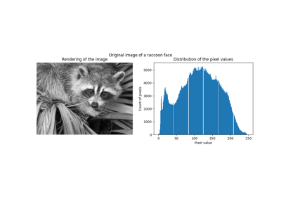
比较使用First Online重建浣熊脸图像含噪碎片的效果的例子字典学习以及各种转化方法。

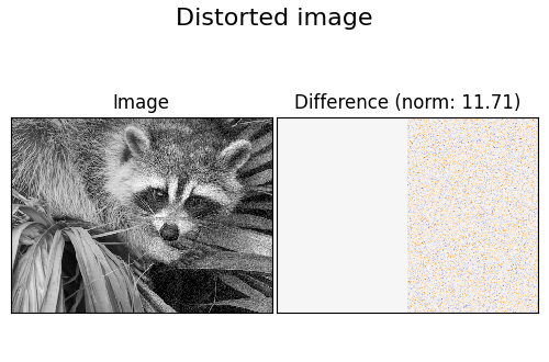
该字典被安装在失真的图像的左半部分上，随后用于重建右半部分。请注意，通过适应未失真（即无噪音）的图像可以获得更好的性能，但这里我们从它不可用的假设开始。

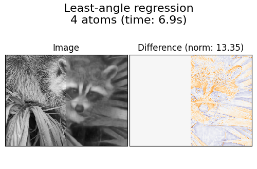
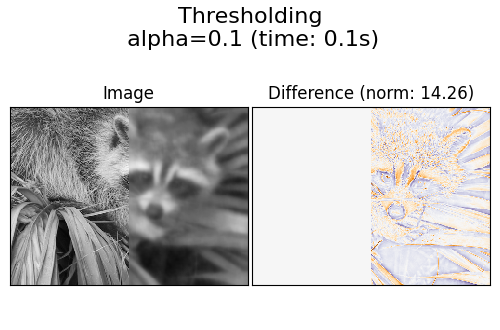
评估图像去噪结果的常见做法是查看重建图像与原始图像之间的差异。如果重建是完美的，这将看起来像高斯噪音。

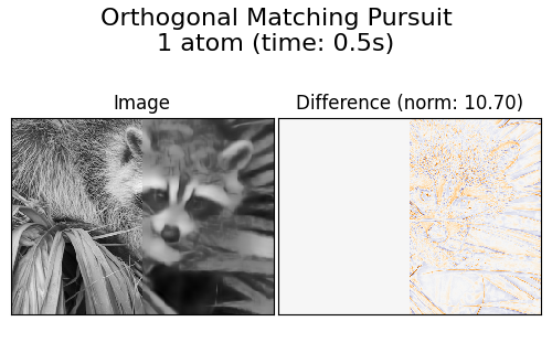
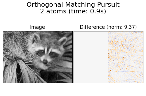
从图中可以看出，垂直匹配追求（OMP）具有两个非零系数的偏差比仅保留一个非零系数时要小一些（边缘看起来不那么突出）。此外，它更接近弗罗贝尼乌斯规范中的基本事实。

的结果最小角回归具有更强的偏见：该差异让人想起原始图像的局部强度值。

采样保持显然对去噪没有用处，但它在这里表明它可以以非常高的速度产生提示性的输出，因此对其他任务（如对象分类）有用，其中性能不一定与可视化相关。

# Authors: The scikit-learn developers
# SPDX-License-Identifier: BSD-3-Clause

生成失真图像#

import numpy as np

try:  # Scipy >= 1.10
    from scipy.datasets import face
except ImportError:
    from scipy.misc import face

raccoon_face = face(gray=True)

# Convert from uint8 representation with values between 0 and 255 to
# a floating point representation with values between 0 and 1.
raccoon_face = raccoon_face / 255.0

# downsample for higher speed
raccoon_face = (
    raccoon_face[::4, ::4]
    + raccoon_face[1::4, ::4]
    + raccoon_face[::4, 1::4]
    + raccoon_face[1::4, 1::4]
)
raccoon_face /= 4.0
height, width = raccoon_face.shape

# Distort the right half of the image
print("Distorting image...")
distorted = raccoon_face.copy()
distorted[:, width // 2 :] += 0.075 * np.random.randn(height, width // 2)

Distorting image...

显示失真图像#

import matplotlib.pyplot as plt


def show_with_diff(image, reference, title):
    """Helper function to display denoising"""
    plt.figure(figsize=(5, 3.3))
    plt.subplot(1, 2, 1)
    plt.title("Image")
    plt.imshow(image, vmin=0, vmax=1, cmap=plt.cm.gray, interpolation="nearest")
    plt.xticks(())
    plt.yticks(())
    plt.subplot(1, 2, 2)
    difference = image - reference

    plt.title("Difference (norm: %.2f)" % np.sqrt(np.sum(difference**2)))
    plt.imshow(
        difference, vmin=-0.5, vmax=0.5, cmap=plt.cm.PuOr, interpolation="nearest"
    )
    plt.xticks(())
    plt.yticks(())
    plt.suptitle(title, size=16)
    plt.subplots_adjust(0.02, 0.02, 0.98, 0.79, 0.02, 0.2)


show_with_diff(distorted, raccoon_face, "Distorted image")

Distorted image, Image, Difference (norm: 11.71)

提取参考补丁#

from time import time

from sklearn.feature_extraction.image import extract_patches_2d

# Extract all reference patches from the left half of the image
print("Extracting reference patches...")
t0 = time()
patch_size = (7, 7)
data = extract_patches_2d(distorted[:, : width // 2], patch_size)
data = data.reshape(data.shape[0], -1)
data -= np.mean(data, axis=0)
data /= np.std(data, axis=0)
print(f"{data.shape[0]} patches extracted in %.2fs." % (time() - t0))

Extracting reference patches...
22692 patches extracted in 0.01s.

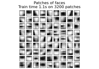
从参考补丁学习词典#

from sklearn.decomposition import MiniBatchDictionaryLearning

print("Learning the dictionary...")
t0 = time()
dico = MiniBatchDictionaryLearning(
    # increase to 300 for higher quality results at the cost of slower
    # training times.
    n_components=50,
    batch_size=200,
    alpha=1.0,
    max_iter=10,
)
V = dico.fit(data).components_
dt = time() - t0
print(f"{dico.n_iter_} iterations / {dico.n_steps_} steps in {dt:.2f}.")

plt.figure(figsize=(4.2, 4))
for i, comp in enumerate(V[:100]):
    plt.subplot(10, 10, i + 1)
    plt.imshow(comp.reshape(patch_size), cmap=plt.cm.gray_r, interpolation="nearest")
    plt.xticks(())
    plt.yticks(())
plt.suptitle(
    "Dictionary learned from face patches\n"
    + "Train time %.1fs on %d patches" % (dt, len(data)),
    fontsize=16,
)
plt.subplots_adjust(0.08, 0.02, 0.92, 0.85, 0.08, 0.23)

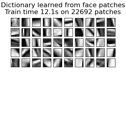
Dictionary learned from face patches Train time 12.1s on 22692 patches

Learning the dictionary...
2.0 iterations / 125 steps in 12.09.

提取有噪的补丁并使用字典重建它们#

from sklearn.feature_extraction.image import reconstruct_from_patches_2d

print("Extracting noisy patches... ")
t0 = time()
data = extract_patches_2d(distorted[:, width // 2 :], patch_size)
data = data.reshape(data.shape[0], -1)
intercept = np.mean(data, axis=0)
data -= intercept
print("done in %.2fs." % (time() - t0))

transform_algorithms = [
    ("Orthogonal Matching Pursuit\n1 atom", "omp", {"transform_n_nonzero_coefs": 1}),
    ("Orthogonal Matching Pursuit\n2 atoms", "omp", {"transform_n_nonzero_coefs": 2}),
    ("Least-angle regression\n4 atoms", "lars", {"transform_n_nonzero_coefs": 4}),
    ("Thresholding\n alpha=0.1", "threshold", {"transform_alpha": 0.1}),
]

reconstructions = {}
for title, transform_algorithm, kwargs in transform_algorithms:
    print(title + "...")
    reconstructions[title] = raccoon_face.copy()
    t0 = time()
    dico.set_params(transform_algorithm=transform_algorithm, **kwargs)
    code = dico.transform(data)
    patches = np.dot(code, V)

    patches += intercept
    patches = patches.reshape(len(data), *patch_size)
    if transform_algorithm == "threshold":
        patches -= patches.min()
        patches /= patches.max()
    reconstructions[title][:, width // 2 :] = reconstruct_from_patches_2d(
        patches, (height, width // 2)
    )
    dt = time() - t0
    print("done in %.2fs." % dt)
    show_with_diff(reconstructions[title], raccoon_face, title + " (time: %.1fs)" % dt)

plt.show()

Extracting noisy patches...
done in 0.00s.
Orthogonal Matching Pursuit
1 atom...
done in 0.50s.
Orthogonal Matching Pursuit
2 atoms...
done in 0.94s.
Least-angle regression
4 atoms...
done in 6.91s.
Thresholding
 alpha=0.1...
done in 0.12s.

Total running time of the script: （0分21.271秒）