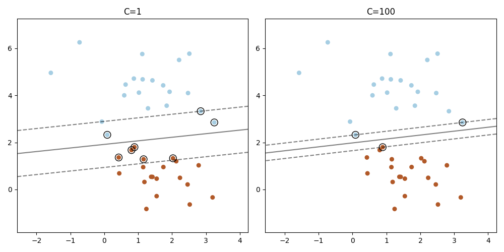
在LinearSRC中绘制支持载体#

与SRC（基于LIBVAR）不同，LinearSRC（基于LIBLININE）不提供支持载体。此示例演示如何在LinearSRC中获取支持载体。

# Authors: The scikit-learn developers
# SPDX-License-Identifier: BSD-3-Clause

import matplotlib.pyplot as plt
import numpy as np

from sklearn.datasets import make_blobs
from sklearn.inspection import DecisionBoundaryDisplay
from sklearn.svm import LinearSVC

X, y = make_blobs(n_samples=40, centers=2, random_state=0)

plt.figure(figsize=(10, 5))
for i, C in enumerate([1, 100]):
    # "hinge" is the standard SVM loss
    clf = LinearSVC(C=C, loss="hinge", random_state=42).fit(X, y)
    # obtain the support vectors through the decision function
    decision_function = clf.decision_function(X)
    # we can also calculate the decision function manually
    # decision_function = np.dot(X, clf.coef_[0]) + clf.intercept_[0]
    # The support vectors are the samples that lie within the margin
    # boundaries, whose size is conventionally constrained to 1
    support_vector_indices = (np.abs(decision_function) <= 1 + 1e-15).nonzero()[0]
    support_vectors = X[support_vector_indices]

    plt.subplot(1, 2, i + 1)
    plt.scatter(X[:, 0], X[:, 1], c=y, s=30, cmap=plt.cm.Paired)
    ax = plt.gca()
    DecisionBoundaryDisplay.from_estimator(
        clf,
        X,
        ax=ax,
        grid_resolution=50,
        plot_method="contour",
        colors="k",
        levels=[-1, 0, 1],
        alpha=0.5,
        linestyles=["--", "-", "--"],
    )
    plt.scatter(
        support_vectors[:, 0],
        support_vectors[:, 1],
        s=100,
        linewidth=1,
        facecolors="none",
        edgecolors="k",
    )
    plt.title("C=" + str(C))
plt.tight_layout()
plt.show()

Total running time of the script: （0分0.133秒）