备注
Go to the end 下载完整的示例代码。或者通过浏览器中的MysterLite或Binder运行此示例
时间序列预测的滞后特征#
此示例演示了如何将Polars设计的滞后特征用于时间序列预测 HistGradientBoostingRegressor 自行车共享需求数据集上。
请参阅上的示例 与时间相关的特征工程 对该数据集进行一些数据探索,并进行定期特征工程演示。
# Authors: The scikit-learn developers
# SPDX-License-Identifier: BSD-3-Clause
分析自行车共享需求数据集#
我们首先从OpenML存储库中加载数据作为原始拼花文件,以说明如何处理任意拼花文件,而不是将这一步骤隐藏在方便工具中,例如 sklearn.datasets.fetch_openml .
拼花文件的URL可以在openml.org(https://www.example.com)openml.org/search?类型=数据&状态=活动& id=44063)。
的 sha256 还提供文件的哈希值以确保下载文件的完整性。
import numpy as np
import polars as pl

from sklearn.datasets import fetch_file

pl.Config.set_fmt_str_lengths(20)

bike_sharing_data_file = fetch_file(
    "https://data.openml.org/datasets/0004/44063/dataset_44063.pq",
    sha256="d120af76829af0d256338dc6dd4be5df4fd1f35bf3a283cab66a51c1c6abd06a",
)
bike_sharing_data_file
PosixPath('/home/bk/scikit_learn_data/data.openml.org/datasets_0004_44063/dataset_44063.pq')
我们用Polars加载拼花地板文件以进行特征工程。Polars自动缓存在多个表达中重复使用的常见子表达(例如 pl.col("count").shift(1) 下面)。请访问https://docs.pola.rs/user-guide/lazy/optimizations/了解更多信息。
df = pl.read_parquet(bike_sharing_data_file)
接下来,我们查看数据集的统计摘要,以便我们可以更好地理解我们正在处理的数据。
import polars.selectors as cs

summary = df.select(cs.numeric()).describe()
summary
让我们看看季节的计数 "fall" , "spring" , "summer" 和 "winter" 以确认它们是平衡的。
import matplotlib.pyplot as plt

df["season"].value_counts()
生成Polar工程的滞后功能#
让我们考虑在给定过去需求的情况下预测下一小时需求的问题。由于需求是一个连续变量,人们可以直观地使用任何回归模型。然而,我们没有通常的 (X_train, y_train) 数据集。相反,我们只有 y_train 按时间顺序组织的需求数据。
lagged_df = df.select(
    "count",
    *[pl.col("count").shift(i).alias(f"lagged_count_{i}h") for i in [1, 2, 3]],
    lagged_count_1d=pl.col("count").shift(24),
    lagged_count_1d_1h=pl.col("count").shift(24 + 1),
    lagged_count_7d=pl.col("count").shift(7 * 24),
    lagged_count_7d_1h=pl.col("count").shift(7 * 24 + 1),
    lagged_mean_24h=pl.col("count").shift(1).rolling_mean(24),
    lagged_max_24h=pl.col("count").shift(1).rolling_max(24),
    lagged_min_24h=pl.col("count").shift(1).rolling_min(24),
    lagged_mean_7d=pl.col("count").shift(1).rolling_mean(7 * 24),
    lagged_max_7d=pl.col("count").shift(1).rolling_max(7 * 24),
    lagged_min_7d=pl.col("count").shift(1).rolling_min(7 * 24),
)
lagged_df.tail(10)
但是请注意,第一行的值未定义,因为它们自己的过去是未知的。这取决于我们使用了多少延迟:
lagged_df.head(10)
我们现在可以在矩阵中分离滞后要素 X 和目标变量(要预测的计数)处于相同第一维度的数组中 y .
lagged_df = lagged_df.drop_nulls()
X = lagged_df.drop("count")
y = lagged_df["count"]
print("X shape: {}\ny shape: {}".format(X.shape, y.shape))
X shape: (17210, 13)
y shape: (17210,)
对下一个小时自行车需求回归的天真评估#
让我们随机分割表格化的数据集来训练梯度增强回归树(GBRT)模型,并使用平均绝对百分比误差(MAPE)对其进行评估。如果我们的模型旨在预测(即,从过去的数据预测未来的数据),我们不应该使用与测试数据无关的训练数据。在时间序列机器学习中,“i.i.d”(独立且同分布)假设并不成立,因为数据点不是独立的并且具有时间关系。
from sklearn.ensemble import HistGradientBoostingRegressor
from sklearn.model_selection import train_test_split

X_train, X_test, y_train, y_test = train_test_split(
    X, y, test_size=0.2, random_state=42
)

model = HistGradientBoostingRegressor().fit(X_train, y_train)
看看模型的性能。
from sklearn.metrics import mean_absolute_percentage_error

y_pred = model.predict(X_test)
mean_absolute_percentage_error(y_test, y_pred)
0.3889873516666431
正确的下一小时预测评估#
让我们使用适当的评估分割策略,考虑数据集的时间结构,以评估我们的模型预测未来数据点的能力(以避免通过读取训练集中滞后特征的值来作弊)。
from sklearn.model_selection import TimeSeriesSplit

ts_cv = TimeSeriesSplit(
    n_splits=3,  # to keep the notebook fast enough on common laptops
    gap=48,  # 2 days data gap between train and test
    max_train_size=10000,  # keep train sets of comparable sizes
    test_size=3000,  # for 2 or 3 digits of precision in scores
)
all_splits = list(ts_cv.split(X, y))
基于MAPE训练模型并评估其性能。
train_idx, test_idx = all_splits[0]
X_train, X_test = X[train_idx, :], X[test_idx, :]
y_train, y_test = y[train_idx], y[test_idx]

model = HistGradientBoostingRegressor().fit(X_train, y_train)
y_pred = model.predict(X_test)
mean_absolute_percentage_error(y_test, y_pred)
0.44300751539296973
通过洗牌训练测试拆分测量的概括误差过于乐观。通过基于时间的拆分进行的概括可能更能代表回归模型的真实性能。让我们通过适当的交叉验证来评估错误评估的变异性:
from sklearn.model_selection import cross_val_score

cv_mape_scores = -cross_val_score(
    model, X, y, cv=ts_cv, scoring="neg_mean_absolute_percentage_error"
)
cv_mape_scores
array([0.44300752, 0.27772182, 0.3697178 ])
拆分之间的可变性相当大!在现实生活中,建议使用更多的分割来更好地评估变异性。从现在开始,让我们报告平均CV分数及其标准差。
print(f"CV MAPE: {cv_mape_scores.mean():.3f} ± {cv_mape_scores.std():.3f}")
CV MAPE: 0.363 ± 0.068
我们可以计算评估指标和损失函数的几种组合,以下将报告这些组合。
from collections import defaultdict

from sklearn.metrics import (
    make_scorer,
    mean_absolute_error,
    mean_pinball_loss,
    root_mean_squared_error,
)
from sklearn.model_selection import cross_validate


def consolidate_scores(cv_results, scores, metric):
    if metric == "MAPE":
        scores[metric].append(f"{value.mean():.2f} ± {value.std():.2f}")
    else:
        scores[metric].append(f"{value.mean():.1f} ± {value.std():.1f}")

    return scores


scoring = {
    "MAPE": make_scorer(mean_absolute_percentage_error),
    "RMSE": make_scorer(root_mean_squared_error),
    "MAE": make_scorer(mean_absolute_error),
    "pinball_loss_05": make_scorer(mean_pinball_loss, alpha=0.05),
    "pinball_loss_50": make_scorer(mean_pinball_loss, alpha=0.50),
    "pinball_loss_95": make_scorer(mean_pinball_loss, alpha=0.95),
}
loss_functions = ["squared_error", "poisson", "absolute_error"]
scores = defaultdict(list)
for loss_func in loss_functions:
    model = HistGradientBoostingRegressor(loss=loss_func)
    cv_results = cross_validate(
        model,
        X,
        y,
        cv=ts_cv,
        scoring=scoring,
        n_jobs=2,
    )
    time = cv_results["fit_time"]
    scores["loss"].append(loss_func)
    scores["fit_time"].append(f"{time.mean():.2f} ± {time.std():.2f} s")

    for key, value in cv_results.items():
        if key.startswith("test_"):
            metric = key.split("test_")[1]
            scores = consolidate_scores(cv_results, scores, metric)
通过分位数回归建模预测不确定性#
而不是对分布的期望值进行建模 \(Y|X\) 就像最小平方和Poisson损失一样,可以尝试估计条件分布的分位数。
\(Y|X=x_i\) 对于给定的数据点, \(x_i\) 因为我们预期租赁的数量不能从特征100%准确地预测。它可能受到现有滞后特征未正确捕获的其他变量的影响。例如,下一个小时是否会下雨,无法从过去几个小时的自行车租赁数据中完全预测。这就是我们所说的任意不确定性。
分位数回归使得可以对该分布进行更好的描述,而无需对其形状做出强烈假设。
quantile_list = [0.05, 0.5, 0.95]

for quantile in quantile_list:
    model = HistGradientBoostingRegressor(loss="quantile", quantile=quantile)
    cv_results = cross_validate(
        model,
        X,
        y,
        cv=ts_cv,
        scoring=scoring,
        n_jobs=2,
    )
    time = cv_results["fit_time"]
    scores["fit_time"].append(f"{time.mean():.2f} ± {time.std():.2f} s")

    scores["loss"].append(f"quantile {int(quantile * 100)}")
    for key, value in cv_results.items():
        if key.startswith("test_"):
            metric = key.split("test_")[1]
            scores = consolidate_scores(cv_results, scores, metric)

scores_df = pl.DataFrame(scores)
scores_df
让我们来看看最小化每个指标的损失。
def min_arg(col):
    col_split = pl.col(col).str.split(" ")
    return pl.arg_sort_by(
        col_split.list.get(0).cast(pl.Float64),
        col_split.list.get(2).cast(pl.Float64),
    ).first()


scores_df.select(
    pl.col("loss").get(min_arg(col_name)).alias(col_name)
    for col_name in scores_df.columns
    if col_name != "loss"
)
即使分数分布因数据集的方差而重叠,当 loss="squared_error" ,而当 loss="absolute_error" 果然分位数5和95的平均弹球损失也是如此。与50分位数损失对应的分数与通过最小化其他损失函数获得的分数重叠,MAE的情况也是如此。
对预测的定性研究#
我们现在可以可视化模型在第5百分位数、中位数和第95百分位数方面的性能:
all_splits = list(ts_cv.split(X, y))
train_idx, test_idx = all_splits[0]

X_train, X_test = X[train_idx, :], X[test_idx, :]
y_train, y_test = y[train_idx], y[test_idx]

max_iter = 50
gbrt_mean_poisson = HistGradientBoostingRegressor(loss="poisson", max_iter=max_iter)
gbrt_mean_poisson.fit(X_train, y_train)
mean_predictions = gbrt_mean_poisson.predict(X_test)

gbrt_median = HistGradientBoostingRegressor(
    loss="quantile", quantile=0.5, max_iter=max_iter
)
gbrt_median.fit(X_train, y_train)
median_predictions = gbrt_median.predict(X_test)

gbrt_percentile_5 = HistGradientBoostingRegressor(
    loss="quantile", quantile=0.05, max_iter=max_iter
)
gbrt_percentile_5.fit(X_train, y_train)
percentile_5_predictions = gbrt_percentile_5.predict(X_test)

gbrt_percentile_95 = HistGradientBoostingRegressor(
    loss="quantile", quantile=0.95, max_iter=max_iter
)
gbrt_percentile_95.fit(X_train, y_train)
percentile_95_predictions = gbrt_percentile_95.predict(X_test)
我们现在可以看看回归模型做出的预测:
last_hours = slice(-96, None)
fig, ax = plt.subplots(figsize=(15, 7))
plt.title("Predictions by regression models")
ax.plot(
    y_test[last_hours],
    "x-",
    alpha=0.2,
    label="Actual demand",
    color="black",
)
ax.plot(
    median_predictions[last_hours],
    "^-",
    label="GBRT median",
)
ax.plot(
    mean_predictions[last_hours],
    "x-",
    label="GBRT mean (Poisson)",
)
ax.fill_between(
    np.arange(96),
    percentile_5_predictions[last_hours],
    percentile_95_predictions[last_hours],
    alpha=0.3,
    label="GBRT 90% interval",
)
_ = ax.legend()

这里有趣的是,5%和95%百分位估计值之间的蓝色区域的宽度随时间而变化:
到了晚上,蓝色带要窄得多:这对车型相当肯定会有少量自行车租赁。此外,这些似乎是正确的,因为实际需求保持在蓝色带内。
白天,蓝色带要宽得多:不确定性增加,可能是因为天气的变异性会产生非常大的影响,尤其是在周末。
我们还可以看到,在工作日,通勤模式在5%和95%的估计中仍然可见。
最后,预计10%的情况下,实际需求不会介于5%和95%百分位估计之间。在这个测试范围内,实际需求似乎更高,尤其是在高峰时段。这可能表明,我们的95%百分位估计低估了需求峰值。这可以通过计算经验覆盖率(如在 calibration of confidence intervals .
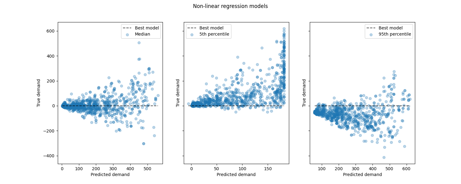
查看非线性回归模型与最佳模型的性能:
from sklearn.metrics import PredictionErrorDisplay

fig, axes = plt.subplots(ncols=3, figsize=(15, 6), sharey=True)
fig.suptitle("Non-linear regression models")
predictions = [
    median_predictions,
    percentile_5_predictions,
    percentile_95_predictions,
]
labels = [
    "Median",
    "5th percentile",
    "95th percentile",
]
for ax, pred, label in zip(axes, predictions, labels):
    PredictionErrorDisplay.from_predictions(
        y_true=y_test,
        y_pred=pred,
        kind="residual_vs_predicted",
        scatter_kwargs={"alpha": 0.3},
        ax=ax,
    )
    ax.set(xlabel="Predicted demand", ylabel="True demand")
    ax.legend(["Best model", label])

plt.show()
结论#
通过这个例子,我们探索了使用滞后特征的时间序列预测。我们比较了朴素回归(使用标准化 train_test_split )采用适当的时间序列评估策略, TimeSeriesSplit .我们观察到该模型使用 train_test_split ,默认值为 shuffle set to True produced an overly optimistic Mean Average Percentage Error (MAPE). The results produced from the time-based split better represent the performance of our time-series regression model. We also analyzed the predictive uncertainty of our model via Quantile Regression. Predictions based on the 5th and 95th percentile using loss="quantile" provide us with a quantitative estimate of the uncertainty of the forecasts made by our time series regression model. Uncertainty estimation can also be performed using MAPIE ,它提供了一种基于最近关于保形预测方法的工作的实现,并同时估计任意性和认识性的不确定性。此外,提供的功能 sktime 通过利用循环时间序列预测,可以用于扩展scikit-learn估计器,从而能够动态预测未来值。
Total running time of the script: (0分8.929秒)
相关实例
Gallery generated by Sphinx-Gallery <https://sphinx-gallery.github.io> _