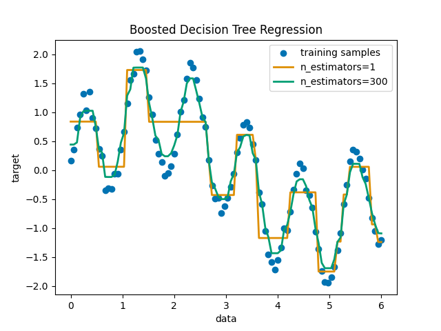
使用AdaBoost进行决策树回归#

使用AdaBoost.R2增强决策树 [1] 在具有少量高斯噪音的1D sin数据集上的算法。将299个增强（300个决策树）与单个决策树回归量进行比较。随着增强次数的增加，回归量可以适应更多细节。

看到梯度增强树的梯度中的功能例如，展示了使用更有效的回归模型（例如 HistGradientBoostingRegressor .

准备数据#

首先，我们准备具有曲线关系和一些高斯噪音的虚拟数据。

# Authors: The scikit-learn developers
# SPDX-License-Identifier: BSD-3-Clause

import numpy as np

rng = np.random.RandomState(1)
X = np.linspace(0, 6, 100)[:, np.newaxis]
y = np.sin(X).ravel() + np.sin(6 * X).ravel() + rng.normal(0, 0.1, X.shape[0])

使用DecisionTree和AdaBoost Regressors进行训练和预测#

现在，我们定义分类器并将其与数据匹配。然后我们对相同的数据进行预测，看看它们能适应多少。第一个回归量是 DecisionTreeRegressor 与 max_depth=4 .第二个回归变量是 AdaBoostRegressor 与 DecisionTreeRegressor 的 max_depth=4 作为基础学习者，并将与 n_estimators=300 这些基础学习者。

from sklearn.ensemble import AdaBoostRegressor
from sklearn.tree import DecisionTreeRegressor

regr_1 = DecisionTreeRegressor(max_depth=4)

regr_2 = AdaBoostRegressor(
    DecisionTreeRegressor(max_depth=4), n_estimators=300, random_state=rng
)

regr_1.fit(X, y)
regr_2.fit(X, y)

y_1 = regr_1.predict(X)
y_2 = regr_2.predict(X)

绘制结果#

最后，我们绘制了我们的两个回归量（单决策树回归量和AdaBoost回归量）对数据的适应程度。

import matplotlib.pyplot as plt
import seaborn as sns

colors = sns.color_palette("colorblind")

plt.figure()
plt.scatter(X, y, color=colors[0], label="training samples")
plt.plot(X, y_1, color=colors[1], label="n_estimators=1", linewidth=2)
plt.plot(X, y_2, color=colors[2], label="n_estimators=300", linewidth=2)
plt.xlabel("data")
plt.ylabel("target")
plt.title("Boosted Decision Tree Regression")
plt.legend()
plt.show()

Total running time of the script: （0分0.367秒）