随机投影嵌入的Johnson-Lindenstrauss界#

的 Johnson-Lindenstrauss lemma 指出任何高维数据集都可以随机投影到低维欧氏空间中，同时控制成对距离的失真。

# Authors: The scikit-learn developers
# SPDX-License-Identifier: BSD-3-Clause

import sys
from time import time

import matplotlib.pyplot as plt
import numpy as np

from sklearn.datasets import fetch_20newsgroups_vectorized, load_digits
from sklearn.metrics.pairwise import euclidean_distances
from sklearn.random_projection import (
    SparseRandomProjection,
    johnson_lindenstrauss_min_dim,
)

理论性能边界#

随机投影引入的失真 p 事实证明， p 正在以良好的概率定义eps嵌入，定义如下：

\[(1 - eps) \|u - v\|^2 < \|p(u) - p(v)\|^2 < (1 + eps) \|u - v\|^2\]

哪里 u 和 v 是从形状数据集中获取的任何行 (n_samples, n_features) 和 p 是一个随机高斯分布的投影 N(0, 1) 形状矩阵 (n_components, n_features) (or稀疏Achlioptas矩阵）。

保证eps嵌入的最小组件数量由下式给出：

\[n\_组件\geq 4 log（n\_样本）/（eps#2/ 2 -eps#3/ 3）\]

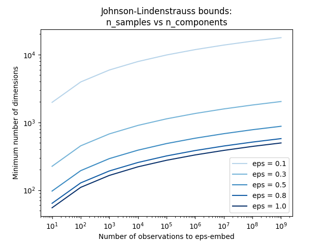
第一个图显示，随着样本数量的增加 n_samples ，最少的维度数量 n_components 为保证 eps - 嵌入。

# range of admissible distortions
eps_range = np.linspace(0.1, 0.99, 5)
colors = plt.cm.Blues(np.linspace(0.3, 1.0, len(eps_range)))

# range of number of samples (observation) to embed
n_samples_range = np.logspace(1, 9, 9)

plt.figure()
for eps, color in zip(eps_range, colors):
    min_n_components = johnson_lindenstrauss_min_dim(n_samples_range, eps=eps)
    plt.loglog(n_samples_range, min_n_components, color=color)

plt.legend([f"eps = {eps:0.1f}" for eps in eps_range], loc="lower right")
plt.xlabel("Number of observations to eps-embed")
plt.ylabel("Minimum number of dimensions")
plt.title("Johnson-Lindenstrauss bounds:\nn_samples vs n_components")
plt.show()

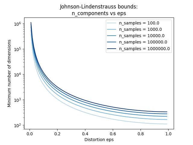
Johnson-Lindenstrauss bounds: n_samples vs n_components

第二个图表明，允许失真的增加 eps 允许大幅减少最少的维度数量 n_components 对于给定数量的样本 n_samples

# range of admissible distortions
eps_range = np.linspace(0.01, 0.99, 100)

# range of number of samples (observation) to embed
n_samples_range = np.logspace(2, 6, 5)
colors = plt.cm.Blues(np.linspace(0.3, 1.0, len(n_samples_range)))

plt.figure()
for n_samples, color in zip(n_samples_range, colors):
    min_n_components = johnson_lindenstrauss_min_dim(n_samples, eps=eps_range)
    plt.semilogy(eps_range, min_n_components, color=color)

plt.legend([f"n_samples = {n}" for n in n_samples_range], loc="upper right")
plt.xlabel("Distortion eps")
plt.ylabel("Minimum number of dimensions")
plt.title("Johnson-Lindenstrauss bounds:\nn_components vs eps")
plt.show()

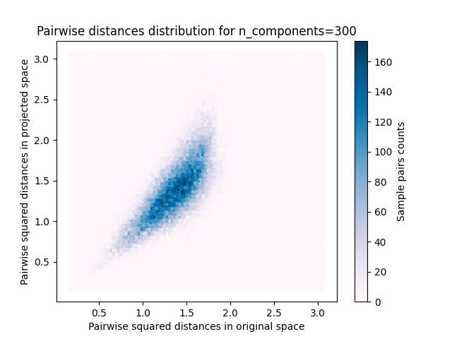
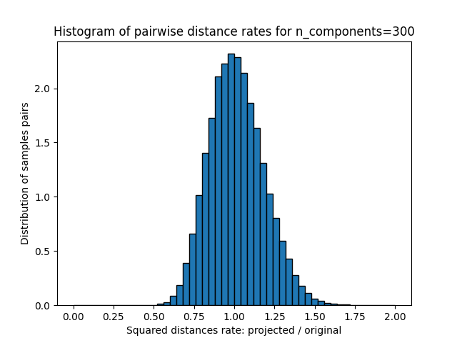
Johnson-Lindenstrauss bounds: n_components vs eps

经验验证#

我们在20个新闻组文本文档（TF-IDF词频）数据集或数字数据集上验证上述界限：

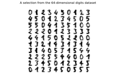
对于20个新闻组数据集，使用稀疏随机矩阵将总共10万个要素的约300个文档投影到较小的欧几里得空间，该空间具有目标维度数的不同值 n_components .
对于数字数据集，300个手写数字图片的一些8 x 8灰度像素数据被随机投影到各种较大维度的空间中 n_components .

默认数据集是20个新闻组数据集。要在数字数据集上运行该示例，请传递 --use-digits-dataset 此脚本的命令行参数。

if "--use-digits-dataset" in sys.argv:
    data = load_digits().data[:300]
else:
    data = fetch_20newsgroups_vectorized().data[:300]

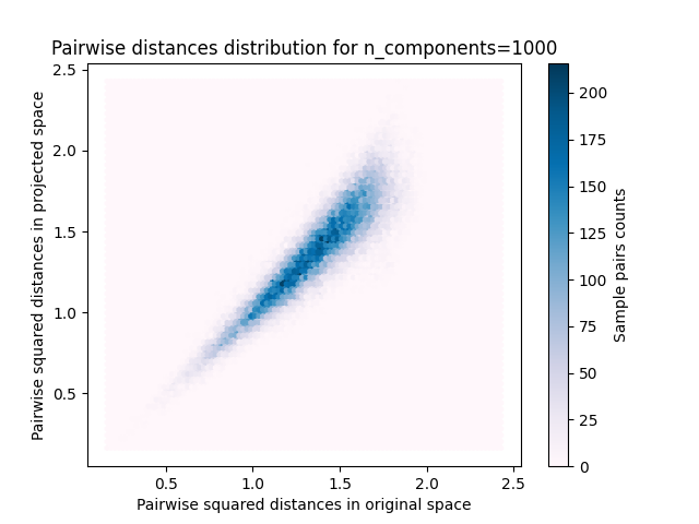
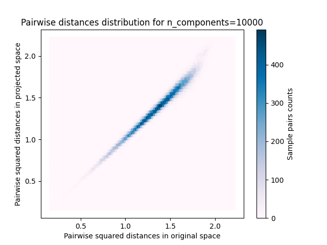
的每个值 n_components ，我们绘制：

样本对的2D分布，原始空间和投影空间中的成对距离分别为x轴和y轴。
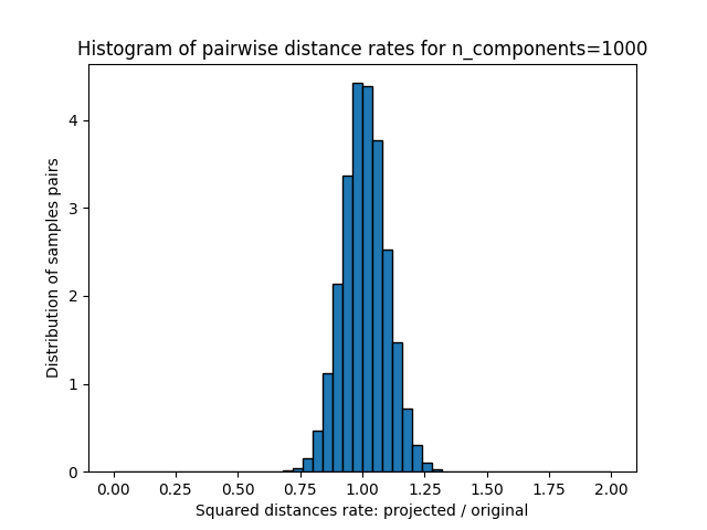
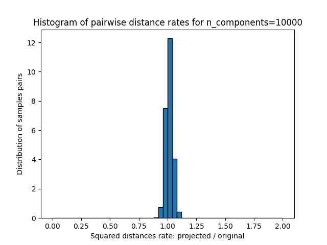
这些距离之比的1D图表（投影/原始）。

n_samples, n_features = data.shape
print(
    f"Embedding {n_samples} samples with dim {n_features} using various "
    "random projections"
)

n_components_range = np.array([300, 1_000, 10_000])
dists = euclidean_distances(data, squared=True).ravel()

# select only non-identical samples pairs
nonzero = dists != 0
dists = dists[nonzero]

for n_components in n_components_range:
    t0 = time()
    rp = SparseRandomProjection(n_components=n_components)
    projected_data = rp.fit_transform(data)
    print(
        f"Projected {n_samples} samples from {n_features} to {n_components} in "
        f"{time() - t0:0.3f}s"
    )
    if hasattr(rp, "components_"):
        n_bytes = rp.components_.data.nbytes
        n_bytes += rp.components_.indices.nbytes
        print(f"Random matrix with size: {n_bytes / 1e6:0.3f} MB")

    projected_dists = euclidean_distances(projected_data, squared=True).ravel()[nonzero]

    plt.figure()
    min_dist = min(projected_dists.min(), dists.min())
    max_dist = max(projected_dists.max(), dists.max())
    plt.hexbin(
        dists,
        projected_dists,
        gridsize=100,
        cmap=plt.cm.PuBu,
        extent=[min_dist, max_dist, min_dist, max_dist],
    )
    plt.xlabel("Pairwise squared distances in original space")
    plt.ylabel("Pairwise squared distances in projected space")
    plt.title("Pairwise distances distribution for n_components=%d" % n_components)
    cb = plt.colorbar()
    cb.set_label("Sample pairs counts")

    rates = projected_dists / dists
    print(f"Mean distances rate: {np.mean(rates):.2f} ({np.std(rates):.2f})")

    plt.figure()
    plt.hist(rates, bins=50, range=(0.0, 2.0), edgecolor="k", density=True)
    plt.xlabel("Squared distances rate: projected / original")
    plt.ylabel("Distribution of samples pairs")
    plt.title("Histogram of pairwise distance rates for n_components=%d" % n_components)

    # TODO: compute the expected value of eps and add them to the previous plot
    # as vertical lines / region

plt.show()

Embedding 300 samples with dim 130107 using various random projections
Projected 300 samples from 130107 to 300 in 0.310s
Random matrix with size: 1.301 MB
Mean distances rate: 1.02 (0.17)
Projected 300 samples from 130107 to 1000 in 0.882s
Random matrix with size: 4.324 MB
Mean distances rate: 1.01 (0.09)
Projected 300 samples from 130107 to 10000 in 7.199s
Random matrix with size: 43.239 MB
Mean distances rate: 1.01 (0.03)

我们可以看到，对于低价值的 n_components 分布很宽，有许多失真对和倾斜分布（由于左侧零比的硬限制，因为距离总是正值），而对于较大的值 n_components 通过随机投影，失真得到控制，距离得到很好的保留。

言论#

根据JL引理，投影300个样本而没有太多失真将至少需要数千个维度，而无论原始数据集的特征数量如何。

因此，在输入空间中仅具有64个特征的数字数据集上使用随机投影是没有意义的：在这种情况下，它不允许降维。

另一方面，在二十个新闻组中，维度可以从56，436减少到10，000，同时合理地保留成对距离。

Total running time of the script: （0分10.491秒）