使用树木集合的特征转换#

将您的特征转换为更高维的稀疏空间。然后在这些特征上训练线性模型。

首先在训练集中适应一组树（完全随机树、随机森林或梯度增强树）。然后，为集成中每棵树的每片叶子分配新特征空间中的固定任意特征索引。然后以一次性方式编码这些叶子索引。

每个样本都会经过整个系统中每棵树的决策，最终得到每棵树的一片叶子。通过将这些叶子的特征值设置为1，将其他特征值设置为0来编码样本。

然后，生成的Transformer学习了数据的监督、稀疏、高维分类嵌入。

# Authors: The scikit-learn developers
# SPDX-License-Identifier: BSD-3-Clause

首先，我们将创建一个大型数据集并将其分为三组：

训练集成方法的集合，这些方法后来用作特征工程Transformer;
训练线性模型的集合;
一组测试线性模型。

重要的是以这种方式分割数据，以避免泄漏数据的过拟合。

from sklearn.datasets import make_classification
from sklearn.model_selection import train_test_split

X, y = make_classification(n_samples=80_000, random_state=10)

X_full_train, X_test, y_full_train, y_test = train_test_split(
    X, y, test_size=0.5, random_state=10
)
X_train_ensemble, X_train_linear, y_train_ensemble, y_train_linear = train_test_split(
    X_full_train, y_full_train, test_size=0.5, random_state=10
)

对于每种集成方法，我们将使用10个估计器和3个级别的最大深度。

n_estimators = 10
max_depth = 3

首先，我们将首先在分离的训练集中训练随机森林和梯度提升

from sklearn.ensemble import GradientBoostingClassifier, RandomForestClassifier

random_forest = RandomForestClassifier(
    n_estimators=n_estimators, max_depth=max_depth, random_state=10
)
random_forest.fit(X_train_ensemble, y_train_ensemble)

gradient_boosting = GradientBoostingClassifier(
    n_estimators=n_estimators, max_depth=max_depth, random_state=10
)
_ = gradient_boosting.fit(X_train_ensemble, y_train_ensemble)

注意到 HistGradientBoostingClassifier 远快于 GradientBoostingClassifier 从中间数据集开始 (n_samples >= 10_000 ），而本示例的情况并非如此。

的 RandomTreesEmbedding 是一种无监督的方法，因此不需要独立训练。

from sklearn.ensemble import RandomTreesEmbedding

random_tree_embedding = RandomTreesEmbedding(
    n_estimators=n_estimators, max_depth=max_depth, random_state=0
)

现在，我们将创建三个管道，将上述嵌入用作预处理阶段。

随机树嵌入可以通过逻辑回归直接流水线化，因为它是标准的scikit-learn Transformer。

from sklearn.linear_model import LogisticRegression
from sklearn.pipeline import make_pipeline

rt_model = make_pipeline(random_tree_embedding, LogisticRegression(max_iter=1000))
rt_model.fit(X_train_linear, y_train_linear)

Pipeline(steps=[('randomtreesembedding',
                 RandomTreesEmbedding(max_depth=3, n_estimators=10,
                                      random_state=0)),
                ('logisticregression', LogisticRegression(max_iter=1000))])

In a Jupyter environment, please rerun this cell to show the HTML representation or trust the notebook.
On GitHub, the HTML representation is unable to render, please try loading this page with nbviewer.org.

然后，我们可以通过逻辑回归管道随机森林或梯度提升。但是，要素转换将通过调用方法进行 apply . scikit-learn中的管道预计接到电话 transform .因此，我们将调用包装为 apply 内 FunctionTransformer .

from sklearn.preprocessing import FunctionTransformer, OneHotEncoder


def rf_apply(X, model):
    return model.apply(X)


rf_leaves_yielder = FunctionTransformer(rf_apply, kw_args={"model": random_forest})

rf_model = make_pipeline(
    rf_leaves_yielder,
    OneHotEncoder(handle_unknown="ignore"),
    LogisticRegression(max_iter=1000),
)
rf_model.fit(X_train_linear, y_train_linear)

Pipeline(steps=[('functiontransformer',
                 FunctionTransformer(func=<function rf_apply at 0x7fa26f869620>,
                                     kw_args={'model': RandomForestClassifier(max_depth=3,
                                                                              n_estimators=10,
                                                                              random_state=10)})),
                ('onehotencoder', OneHotEncoder(handle_unknown='ignore')),
                ('logisticregression', LogisticRegression(max_iter=1000))])

In a Jupyter environment, please rerun this cell to show the HTML representation or trust the notebook.
On GitHub, the HTML representation is unable to render, please try loading this page with nbviewer.org.

def gbdt_apply(X, model):
    return model.apply(X)[:, :, 0]


gbdt_leaves_yielder = FunctionTransformer(
    gbdt_apply, kw_args={"model": gradient_boosting}
)

gbdt_model = make_pipeline(
    gbdt_leaves_yielder,
    OneHotEncoder(handle_unknown="ignore"),
    LogisticRegression(max_iter=1000),
)
gbdt_model.fit(X_train_linear, y_train_linear)

Pipeline(steps=[('functiontransformer',
                 FunctionTransformer(func=<function gbdt_apply at 0x7fa26f868ae0>,
                                     kw_args={'model': GradientBoostingClassifier(n_estimators=10,
                                                                                  random_state=10)})),
                ('onehotencoder', OneHotEncoder(handle_unknown='ignore')),
                ('logisticregression', LogisticRegression(max_iter=1000))])

In a Jupyter environment, please rerun this cell to show the HTML representation or trust the notebook.
On GitHub, the HTML representation is unable to render, please try loading this page with nbviewer.org.

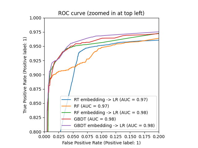
我们最终可以显示所有模型的不同ROC曲线。

import matplotlib.pyplot as plt

from sklearn.metrics import RocCurveDisplay

_, ax = plt.subplots()

models = [
    ("RT embedding -> LR", rt_model),
    ("RF", random_forest),
    ("RF embedding -> LR", rf_model),
    ("GBDT", gradient_boosting),
    ("GBDT embedding -> LR", gbdt_model),
]

model_displays = {}
for name, pipeline in models:
    model_displays[name] = RocCurveDisplay.from_estimator(
        pipeline, X_test, y_test, ax=ax, name=name
    )
_ = ax.set_title("ROC curve")

_, ax = plt.subplots()
for name, pipeline in models:
    model_displays[name].plot(ax=ax)

ax.set_xlim(0, 0.2)
ax.set_ylim(0.8, 1)
_ = ax.set_title("ROC curve (zoomed in at top left)")

Total running time of the script: （0分2.428秒）