scikit-learn 0.24发布亮点#

我们很高兴宣布scikit-learn 0.24的发布！添加了许多错误修复和改进，以及一些新的关键功能。我们在下面详细介绍了该版本的一些主要功能。 For an exhaustive list of all the changes ，请参阅 release notes .

安装最新版本（使用pip）：

pip install --upgrade scikit-learn

或带有conda：：

conda install -c conda-forge scikit-learn

超参数整定的逐次减半估计#

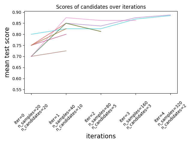
连续减半是一种最先进的方法，现在可以探索参数的空间并确定其最佳组合。 HalvingGridSearchCV 和 HalvingRandomSearchCV 可用作临时替代品 GridSearchCV 和 RandomizedSearchCV .连续减半是一个迭代选择过程，如下图所示。第一次迭代使用少量资源运行，其中资源通常对应于训练样本的数量，但也可以是任意的整参数，例如 n_estimators 在一片随机的森林中。仅为下一次迭代选择参数候选者的一个子集，该迭代将在分配的资源量不断增加的情况下运行。只有候选项的一个子集会持续到迭代过程结束，并且最佳参数候选项是在最后一次迭代中得分最高的参数。

阅读更多的 User Guide (note：连续减半估计值仍然 experimental ).

../../_images/sphx_glr_plot_successive_halving_iterations_001.png

import numpy as np
from scipy.stats import randint

from sklearn.datasets import make_classification
from sklearn.ensemble import RandomForestClassifier
from sklearn.experimental import enable_halving_search_cv  # noqa: F401
from sklearn.model_selection import HalvingRandomSearchCV

rng = np.random.RandomState(0)

X, y = make_classification(n_samples=700, random_state=rng)

clf = RandomForestClassifier(n_estimators=10, random_state=rng)

param_dist = {
    "max_depth": [3, None],
    "max_features": randint(1, 11),
    "min_samples_split": randint(2, 11),
    "bootstrap": [True, False],
    "criterion": ["gini", "entropy"],
}

rsh = HalvingRandomSearchCV(
    estimator=clf, param_distributions=param_dist, factor=2, random_state=rng
)
rsh.fit(X, y)
rsh.best_params_

{'bootstrap': True, 'criterion': 'gini', 'max_depth': None, 'max_features': 10, 'min_samples_split': 10}

对HistorentBoosting估计器中分类特征的本地支持#

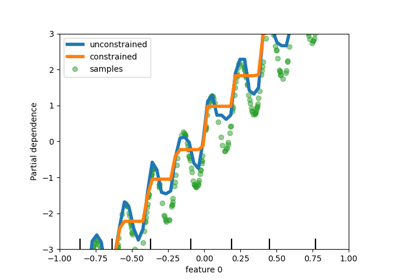
HistGradientBoostingClassifier 和 HistGradientBoostingRegressor 现在有了对分类特征的原生支持：它们可以考虑对无序的分类数据进行拆分。阅读更多的 User Guide .

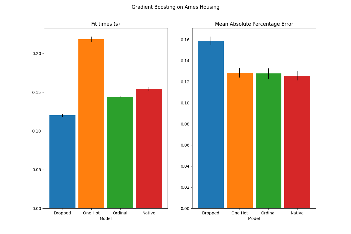
../../_images/sphx_glr_plot_gradient_boosting_categorical_001.png

该图显示，对类别特征的新本地支持导致的匹配时间与类别被视为有序量（即简单地顺序编码）的模型相当。原生支持也比单一热编码和有序编码更具表达力。然而，要使用新的 categorical_features 参数，仍然需要对管道内的数据进行预处理，如本文所示 example .

改进HistorentBoosting估计器的性能#

的内存占用 ensemble.HistGradientBoostingRegressor 和 ensemble.HistGradientBoostingClassifier 在致电期间，情况显着改善 fit. In addition, histogram initialization is now done in parallel which results in slight speed improvements. See more in the Benchmark page .

一种新的自训练元估计器#

一种新的自我训练实现，基于 Yarowski's algorithm 现在可以与任何实现 predict_proba .子分类器将充当半监督分类器，允许它从未标记的数据中学习。阅读更多的 User guide .

import numpy as np

from sklearn import datasets
from sklearn.semi_supervised import SelfTrainingClassifier
from sklearn.svm import SVC

rng = np.random.RandomState(42)
iris = datasets.load_iris()
random_unlabeled_points = rng.rand(iris.target.shape[0]) < 0.3
iris.target[random_unlabeled_points] = -1
svc = SVC(probability=True, gamma="auto")
self_training_model = SelfTrainingClassifier(svc)
self_training_model.fit(iris.data, iris.target)

SelfTrainingClassifier(estimator=SVC(gamma='auto', probability=True))

In a Jupyter environment, please rerun this cell to show the HTML representation or trust the notebook.
On GitHub, the HTML representation is unable to render, please try loading this page with nbviewer.org.

新的SequentialMetureMetrics Transformer#

提供了一个新的迭代Transformer来选择特征： SequentialFeatureSelector .顺序特征选择可以根据交叉验证的分数最大化，一次添加一个特征（向前选择）或从可用特征列表中删除特征（向后选择）。看到 User Guide .

from sklearn.datasets import load_iris
from sklearn.feature_selection import SequentialFeatureSelector
from sklearn.neighbors import KNeighborsClassifier

X, y = load_iris(return_X_y=True, as_frame=True)
feature_names = X.columns
knn = KNeighborsClassifier(n_neighbors=3)
sfs = SequentialFeatureSelector(knn, n_features_to_select=2)
sfs.fit(X, y)
print(
    "Features selected by forward sequential selection: "
    f"{feature_names[sfs.get_support()].tolist()}"
)

Features selected by forward sequential selection: ['sepal length (cm)', 'petal width (cm)']

新的PolynomialCountSketch核逼近函数#

新 PolynomialCountSketch 与线性模型一起使用时，逼近特征空间的多项扩展，但使用的内存比 PolynomialFeatures .

from sklearn.datasets import fetch_covtype
from sklearn.kernel_approximation import PolynomialCountSketch
from sklearn.linear_model import LogisticRegression
from sklearn.model_selection import train_test_split
from sklearn.pipeline import make_pipeline
from sklearn.preprocessing import MinMaxScaler

X, y = fetch_covtype(return_X_y=True)
pipe = make_pipeline(
    MinMaxScaler(),
    PolynomialCountSketch(degree=2, n_components=300),
    LogisticRegression(max_iter=1000),
)
X_train, X_test, y_train, y_test = train_test_split(
    X, y, train_size=5000, test_size=10000, random_state=42
)
pipe.fit(X_train, y_train).score(X_test, y_test)

0.7335

为了进行比较，以下是相同数据的线性基线的得分：

linear_baseline = make_pipeline(MinMaxScaler(), LogisticRegression(max_iter=1000))
linear_baseline.fit(X_train, y_train).score(X_test, y_test)

0.7141

个人条件期望图#

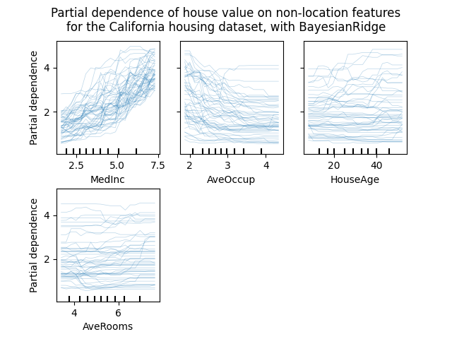
有一种新的部分依赖图可用：个人条件期望（ICE）图。ICE图分别可视化每个样本的预测对特征的依赖性，每个样本有一条线。看到 User Guide

from sklearn.datasets import fetch_california_housing
from sklearn.ensemble import RandomForestRegressor

# from sklearn.inspection import plot_partial_dependence
from sklearn.inspection import PartialDependenceDisplay

X, y = fetch_california_housing(return_X_y=True, as_frame=True)
features = ["MedInc", "AveOccup", "HouseAge", "AveRooms"]
est = RandomForestRegressor(n_estimators=10)
est.fit(X, y)

# plot_partial_dependence has been removed in version 1.2. From 1.2, use
# PartialDependenceDisplay instead.
# display = plot_partial_dependence(
display = PartialDependenceDisplay.from_estimator(
    est,
    X,
    features,
    kind="individual",
    subsample=50,
    n_jobs=3,
    grid_resolution=20,
    random_state=0,
)
display.figure_.suptitle(
    "Partial dependence of house value on non-location features\n"
    "for the California housing dataset, with BayesianRidge"
)
display.figure_.subplots_adjust(hspace=0.3)

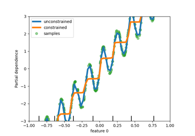
Partial dependence of house value on non-location features for the California housing dataset, with BayesianRidge

一种新的DecisionTreeRegressor Poisson分裂准则#

Poisson回归估计的集成从0.23版本开始继续。 DecisionTreeRegressor 现在支持新的 'poisson' 分裂准则设置 criterion="poisson" 如果您的目标是计数或频率，这可能是一个不错的选择。

import numpy as np

from sklearn.model_selection import train_test_split
from sklearn.tree import DecisionTreeRegressor

n_samples, n_features = 1000, 20
rng = np.random.RandomState(0)
X = rng.randn(n_samples, n_features)
# positive integer target correlated with X[:, 5] with many zeros:
y = rng.poisson(lam=np.exp(X[:, 5]) / 2)
X_train, X_test, y_train, y_test = train_test_split(X, y, random_state=rng)
regressor = DecisionTreeRegressor(criterion="poisson", random_state=0)
regressor.fit(X_train, y_train)

DecisionTreeRegressor(criterion='poisson', random_state=0)

In a Jupyter environment, please rerun this cell to show the HTML representation or trust the notebook.
On GitHub, the HTML representation is unable to render, please try loading this page with nbviewer.org.

新的文档改进#

添加了新的示例和文档页面，以不断努力提高对机器学习实践的理解：

关于 common pitfalls and recommended practices ,
示例说明如何 statistically compare the performance of models 评价使用 GridSearchCV ,
关于如何 interpret coefficients of linear models ,
一个 example 主成分回归和偏最小二乘法的比较

Total running time of the script: （0分15.427秒）