梯度增强回归#

此示例演示梯度提升从弱预测模型集合生成预测模型。梯度提升可用于回归和分类问题。在这里，我们将训练一个模型来处理糖尿病回归任务。我们将从以下方面获得结果： GradientBoostingRegressor 具有最小平方损失和深度为4的500棵回归树。

注：对于更大的数据集（n_samples >= 10000），请参阅 HistGradientBoostingRegressor .看到梯度增强树的梯度中的功能举个例子，展示了 HistGradientBoostingRegressor .

# Authors: The scikit-learn developers
# SPDX-License-Identifier: BSD-3-Clause

import matplotlib
import matplotlib.pyplot as plt
import numpy as np

from sklearn import datasets, ensemble
from sklearn.inspection import permutation_importance
from sklearn.metrics import mean_squared_error
from sklearn.model_selection import train_test_split
from sklearn.utils.fixes import parse_version

加载数据#

首先我们需要加载数据。

diabetes = datasets.load_diabetes()
X, y = diabetes.data, diabetes.target

数据预处理#

接下来，我们将拆分数据集，将90%用于训练，其余部分用于测试。我们还将设置回归模型参数。您可以使用这些参数来查看结果如何变化。

n_estimators ：将执行的升压级的数量。稍后，我们将绘制与提升迭代的偏差。

max_depth ：限制树中的节点数量。最佳值取决于输入变量的相互作用。

min_samples_split ：拆分内部节点所需的最小样本数。

learning_rate ：每棵树的贡献会减少多少。

loss : loss function to optimize. The least squares function is used in this case however, there are many other options (see GradientBoostingRegressor ).

X_train, X_test, y_train, y_test = train_test_split(
    X, y, test_size=0.1, random_state=13
)

params = {
    "n_estimators": 500,
    "max_depth": 4,
    "min_samples_split": 5,
    "learning_rate": 0.01,
    "loss": "squared_error",
}

匹配回归模型#

现在我们将启动梯度增强回归器，并将其与我们的训练数据进行匹配。让我们再看看测试数据的均方误差。

reg = ensemble.GradientBoostingRegressor(**params)
reg.fit(X_train, y_train)

mse = mean_squared_error(y_test, reg.predict(X_test))
print("The mean squared error (MSE) on test set: {:.4f}".format(mse))

The mean squared error (MSE) on test set: 3010.2061

情节训练偏差#

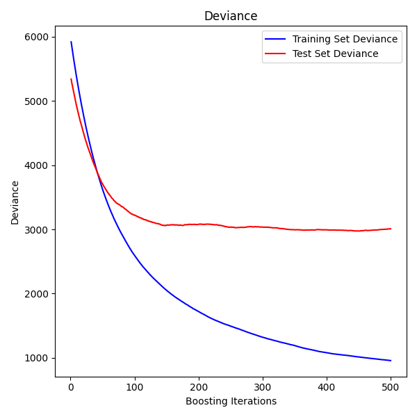
最后，我们将可视化结果。为此，我们将首先计算测试集偏差，然后根据增强迭代绘制它。

test_score = np.zeros((params["n_estimators"],), dtype=np.float64)
for i, y_pred in enumerate(reg.staged_predict(X_test)):
    test_score[i] = mean_squared_error(y_test, y_pred)

fig = plt.figure(figsize=(6, 6))
plt.subplot(1, 1, 1)
plt.title("Deviance")
plt.plot(
    np.arange(params["n_estimators"]) + 1,
    reg.train_score_,
    "b-",
    label="Training Set Deviance",
)
plt.plot(
    np.arange(params["n_estimators"]) + 1, test_score, "r-", label="Test Set Deviance"
)
plt.legend(loc="upper right")
plt.xlabel("Boosting Iterations")
plt.ylabel("Deviance")
fig.tight_layout()
plt.show()

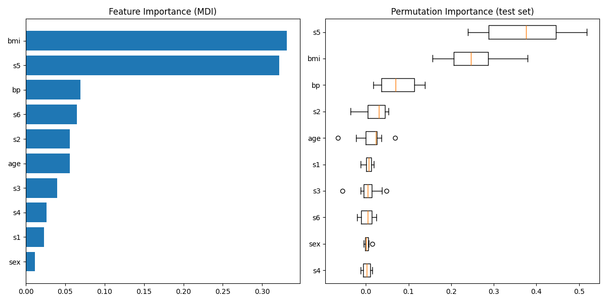
情节特征重要性#

警告

Careful, impurity-based feature importances can be misleading for high cardinality features (many unique values). As an alternative, the permutation importances of reg can be computed on a held out test set. See 排列特征重要性 for more details.

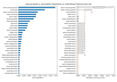
对于本例，基于杂质和排列的方法识别相同的2个强预测特征，但顺序不同。第三个最具预测性的特征“BP”对于这2种方法也是相同的。其余特征的预测性较差，排列图的误差线显示它们与0重叠。

feature_importance = reg.feature_importances_
sorted_idx = np.argsort(feature_importance)
pos = np.arange(sorted_idx.shape[0]) + 0.5
fig = plt.figure(figsize=(12, 6))
plt.subplot(1, 2, 1)
plt.barh(pos, feature_importance[sorted_idx], align="center")
plt.yticks(pos, np.array(diabetes.feature_names)[sorted_idx])
plt.title("Feature Importance (MDI)")

result = permutation_importance(
    reg, X_test, y_test, n_repeats=10, random_state=42, n_jobs=2
)
sorted_idx = result.importances_mean.argsort()
plt.subplot(1, 2, 2)

# `labels` argument in boxplot is deprecated in matplotlib 3.9 and has been
# renamed to `tick_labels`. The following code handles this, but as a
# scikit-learn user you probably can write simpler code by using `labels=...`
# (matplotlib < 3.9) or `tick_labels=...` (matplotlib >= 3.9).
tick_labels_parameter_name = (
    "tick_labels"
    if parse_version(matplotlib.__version__) >= parse_version("3.9")
    else "labels"
)
tick_labels_dict = {
    tick_labels_parameter_name: np.array(diabetes.feature_names)[sorted_idx]
}
plt.boxplot(result.importances[sorted_idx].T, vert=False, **tick_labels_dict)
plt.title("Permutation Importance (test set)")
fig.tight_layout()
plt.show()

Feature Importance (MDI), Permutation Importance (test set)

Total running time of the script: （0分1.202秒）