回归模型中目标转换的效果

在这个例子中，我们概述了 TransformedTargetRegressor .我们使用两个例子来说明在学习线性回归模型之前转换目标的好处。第一个示例使用合成数据，而第二个示例基于Ames住房数据集。

# Authors: The scikit-learn developers
# SPDX-License-Identifier: BSD-3-Clause

print(__doc__)

合成实施例

生成合成随机回归数据集。目标 y 修改者：

1. translating all targets such that all entries are non-negative (by adding the absolute value of the lowest y) and

2. 应用指数函数来获得无法使用简单线性模型进行匹配的非线性目标。

因此，对数 (np.log1p ）和指数函数 (np.expm1 ）将用于在训练线性回归模型并将其用于预测之前转换目标。

import numpy as np

from sklearn.datasets import make_regression

X, y = make_regression(n_samples=10_000, noise=100, random_state=0)
y = np.expm1((y + abs(y.min())) / 200)
y_trans = np.log1p(y)

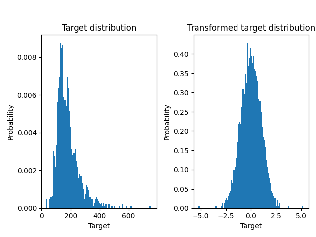
下面我们绘制了应用对数函数之前和之后目标的概率密度函数。

import matplotlib.pyplot as plt

from sklearn.model_selection import train_test_split

f, (ax0, ax1) = plt.subplots(1, 2)

ax0.hist(y, bins=100, density=True)
ax0.set_xlim([0, 2000])
ax0.set_ylabel("Probability")
ax0.set_xlabel("Target")
ax0.set_title("Target distribution")

ax1.hist(y_trans, bins=100, density=True)
ax1.set_ylabel("Probability")
ax1.set_xlabel("Target")
ax1.set_title("Transformed target distribution")

f.suptitle("Synthetic data", y=1.05)
plt.tight_layout()

X_train, X_test, y_train, y_test = train_test_split(X, y, random_state=0)

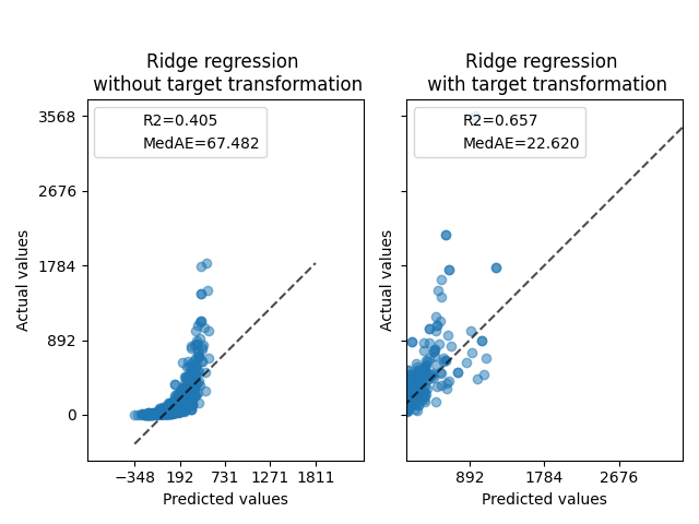
首先，将线性模型应用于原始目标。由于非线性，训练的模型在预测期间不会精确。随后，使用对目标进行线性化，即使使用中位数绝对误差（MedAE）报告的类似线性模型，也可以进行更好的预测。

from sklearn.metrics import median_absolute_error, r2_score


def compute_score(y_true, y_pred):
    return {
        "R2": f"{r2_score(y_true, y_pred):.3f}",
        "MedAE": f"{median_absolute_error(y_true, y_pred):.3f}",
    }

from sklearn.compose import TransformedTargetRegressor
from sklearn.linear_model import RidgeCV
from sklearn.metrics import PredictionErrorDisplay

f, (ax0, ax1) = plt.subplots(1, 2, sharey=True)

ridge_cv = RidgeCV().fit(X_train, y_train)
y_pred_ridge = ridge_cv.predict(X_test)

ridge_cv_with_trans_target = TransformedTargetRegressor(
    regressor=RidgeCV(), func=np.log1p, inverse_func=np.expm1
).fit(X_train, y_train)
y_pred_ridge_with_trans_target = ridge_cv_with_trans_target.predict(X_test)

PredictionErrorDisplay.from_predictions(
    y_test,
    y_pred_ridge,
    kind="actual_vs_predicted",
    ax=ax0,
    scatter_kwargs={"alpha": 0.5},
)
PredictionErrorDisplay.from_predictions(
    y_test,
    y_pred_ridge_with_trans_target,
    kind="actual_vs_predicted",
    ax=ax1,
    scatter_kwargs={"alpha": 0.5},
)

# Add the score in the legend of each axis
for ax, y_pred in zip([ax0, ax1], [y_pred_ridge, y_pred_ridge_with_trans_target]):
    for name, score in compute_score(y_test, y_pred).items():
        ax.plot([], [], " ", label=f"{name}={score}")
    ax.legend(loc="upper left")

ax0.set_title("Ridge regression \n without target transformation")
ax1.set_title("Ridge regression \n with target transformation")
f.suptitle("Synthetic data", y=1.05)
plt.tight_layout()

现实世界数据集

以类似的方式，Ames住房数据集用于显示在学习模型之前转换目标的影响。在本例中，要预测的目标是每套房屋的售价。

from sklearn.datasets import fetch_openml
from sklearn.preprocessing import quantile_transform

ames = fetch_openml(name="house_prices", as_frame=True)
# Keep only numeric columns
X = ames.data.select_dtypes(np.number)
# Remove columns with NaN or Inf values
X = X.drop(columns=["LotFrontage", "GarageYrBlt", "MasVnrArea"])
# Let the price be in k$
y = ames.target / 1000
y_trans = quantile_transform(
    y.to_frame(), n_quantiles=900, output_distribution="normal", copy=True
).squeeze()

A QuantileTransformer 用于在应用 RidgeCV 模型

f, (ax0, ax1) = plt.subplots(1, 2)

ax0.hist(y, bins=100, density=True)
ax0.set_ylabel("Probability")
ax0.set_xlabel("Target")
ax0.set_title("Target distribution")

ax1.hist(y_trans, bins=100, density=True)
ax1.set_ylabel("Probability")
ax1.set_xlabel("Target")
ax1.set_title("Transformed target distribution")

f.suptitle("Ames housing data: selling price", y=1.05)
plt.tight_layout()

X_train, X_test, y_train, y_test = train_test_split(X, y, random_state=1)

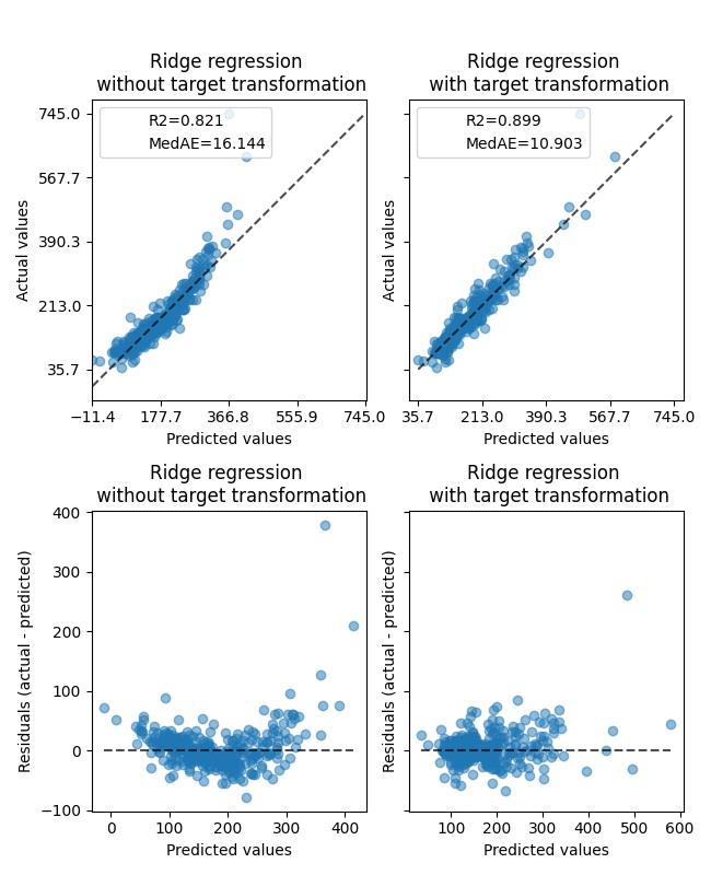
Transformer的影响弱于对合成数据的影响。然而，转变导致 \(R^2\) MedAE大幅下降。没有目标变换的残差图（预测目标-真实目标与预测目标）呈现弯曲的“反向微笑”形状，这是由于残差值根据预测目标的值而变化。通过目标变换，形状更加线性，表明模型拟合更好。

from sklearn.preprocessing import QuantileTransformer

f, (ax0, ax1) = plt.subplots(2, 2, sharey="row", figsize=(6.5, 8))

ridge_cv = RidgeCV().fit(X_train, y_train)
y_pred_ridge = ridge_cv.predict(X_test)

ridge_cv_with_trans_target = TransformedTargetRegressor(
    regressor=RidgeCV(),
    transformer=QuantileTransformer(n_quantiles=900, output_distribution="normal"),
).fit(X_train, y_train)
y_pred_ridge_with_trans_target = ridge_cv_with_trans_target.predict(X_test)

# plot the actual vs predicted values
PredictionErrorDisplay.from_predictions(
    y_test,
    y_pred_ridge,
    kind="actual_vs_predicted",
    ax=ax0[0],
    scatter_kwargs={"alpha": 0.5},
)
PredictionErrorDisplay.from_predictions(
    y_test,
    y_pred_ridge_with_trans_target,
    kind="actual_vs_predicted",
    ax=ax0[1],
    scatter_kwargs={"alpha": 0.5},
)

# Add the score in the legend of each axis
for ax, y_pred in zip([ax0[0], ax0[1]], [y_pred_ridge, y_pred_ridge_with_trans_target]):
    for name, score in compute_score(y_test, y_pred).items():
        ax.plot([], [], " ", label=f"{name}={score}")
    ax.legend(loc="upper left")

ax0[0].set_title("Ridge regression \n without target transformation")
ax0[1].set_title("Ridge regression \n with target transformation")

# plot the residuals vs the predicted values
PredictionErrorDisplay.from_predictions(
    y_test,
    y_pred_ridge,
    kind="residual_vs_predicted",
    ax=ax1[0],
    scatter_kwargs={"alpha": 0.5},
)
PredictionErrorDisplay.from_predictions(
    y_test,
    y_pred_ridge_with_trans_target,
    kind="residual_vs_predicted",
    ax=ax1[1],
    scatter_kwargs={"alpha": 0.5},
)
ax1[0].set_title("Ridge regression \n without target transformation")
ax1[1].set_title("Ridge regression \n with target transformation")

f.suptitle("Ames housing data: selling price", y=1.05)
plt.tight_layout()
plt.show()

相关实例

保序回归

Isotonic Regression

流水线：链接PCA和逻辑回归

Pipelining: chaining a PCA and a logistic regression

使用堆叠组合预测因子

Combine predictors using stacking

绘制交叉验证预测

Plotting Cross-Validated Predictions