比较线性Bayesian回归量#

此示例比较了两个不同的bavoy回归量：

一自动相关性确定- ARD
一 Bayesian Ridge Regression

在第一部分中，我们使用普通最小二乘 (OLS)模型作为基线，用于将模型的系数与真实系数进行比较。此后，我们表明，这样的模型的估计是通过迭代最大化的边际对数似然的观察。

在最后一节中，我们使用多项特征展开来绘制ARD和Bayesian Ridge回归的预测和不确定性，以适应两者之间的非线性关系 X 和 y .

# Authors: The scikit-learn developers
# SPDX-License-Identifier: BSD-3-Clause

模型恢复地面真值权重的稳健性#

生成合成数据集#

我们生成一个数据集， X 和 y 呈线性联系：10个特征 X 将用于生成 y .其他功能对于预测没有用处 y .此外，我们生成一个数据集，其中 n_samples == n_features .这种设置对于OLS模型来说是具有挑战性的，并且可能导致任意的大权重。拥有重量优先权和处罚会加剧问题。最后，添加高斯噪音。

from sklearn.datasets import make_regression

X, y, true_weights = make_regression(
    n_samples=100,
    n_features=100,
    n_informative=10,
    noise=8,
    coef=True,
    random_state=42,
)

适应回归量#

现在，我们对Bayesian模型和OLS进行匹配，以便稍后比较模型的系数。

import pandas as pd

from sklearn.linear_model import ARDRegression, BayesianRidge, LinearRegression

olr = LinearRegression().fit(X, y)
brr = BayesianRidge(compute_score=True, max_iter=30).fit(X, y)
ard = ARDRegression(compute_score=True, max_iter=30).fit(X, y)
df = pd.DataFrame(
    {
        "Weights of true generative process": true_weights,
        "ARDRegression": ard.coef_,
        "BayesianRidge": brr.coef_,
        "LinearRegression": olr.coef_,
    }
)

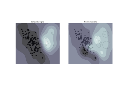
绘制真实系数和估计系数#

现在我们将每个模型的系数与真实生成模型的权重进行比较。

import matplotlib.pyplot as plt
import seaborn as sns
from matplotlib.colors import SymLogNorm

plt.figure(figsize=(10, 6))
ax = sns.heatmap(
    df.T,
    norm=SymLogNorm(linthresh=10e-4, vmin=-80, vmax=80),
    cbar_kws={"label": "coefficients' values"},
    cmap="seismic_r",
)
plt.ylabel("linear model")
plt.xlabel("coefficients")
plt.tight_layout(rect=(0, 0, 1, 0.95))
_ = plt.title("Models' coefficients")

由于增加的噪音，没有一个模型恢复真实权重。事实上，所有模型总是有10个以上的非零系数。与OLS估计器相比，使用Bayesian Ridge回归的系数稍微向零移动，从而使它们稳定。ARD回归提供了一种更稀疏的解决方案：一些非信息系数被完全设置为零，而将其他系数移至更接近零。一些非信息系数仍然存在并保留很大的值。

绘制边际log似然#

import numpy as np

ard_scores = -np.array(ard.scores_)
brr_scores = -np.array(brr.scores_)
plt.plot(ard_scores, color="navy", label="ARD")
plt.plot(brr_scores, color="red", label="BayesianRidge")
plt.ylabel("Log-likelihood")
plt.xlabel("Iterations")
plt.xlim(1, 30)
plt.legend()
_ = plt.title("Models log-likelihood")

事实上，这两个模型都将log似然最小化到由 max_iter 参数.

具有多项特征扩展的Bayesian回归#

生成合成数据集#

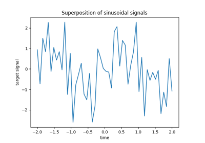
我们创建一个目标，该目标是输入特征的非线性函数。添加遵循标准均匀分布的噪音。

from sklearn.pipeline import make_pipeline
from sklearn.preprocessing import PolynomialFeatures, StandardScaler

rng = np.random.RandomState(0)
n_samples = 110

# sort the data to make plotting easier later
X = np.sort(-10 * rng.rand(n_samples) + 10)
noise = rng.normal(0, 1, n_samples) * 1.35
y = np.sqrt(X) * np.sin(X) + noise
full_data = pd.DataFrame({"input_feature": X, "target": y})
X = X.reshape((-1, 1))

# extrapolation
X_plot = np.linspace(10, 10.4, 10)
y_plot = np.sqrt(X_plot) * np.sin(X_plot)
X_plot = np.concatenate((X, X_plot.reshape((-1, 1))))
y_plot = np.concatenate((y - noise, y_plot))

适应回归量#

Here we try a degree 10 polynomial to potentially overfit, though the bayesian linear models regularize the size of the polynomial coefficients. As fit_intercept=True by default for ARDRegression and BayesianRidge, then PolynomialFeatures should not introduce an additional bias feature. By setting return_std=True, the bayesian regressors return the standard deviation of the posterior distribution for the model parameters.

ard_poly = make_pipeline(
    PolynomialFeatures(degree=10, include_bias=False),
    StandardScaler(),
    ARDRegression(),
).fit(X, y)
brr_poly = make_pipeline(
    PolynomialFeatures(degree=10, include_bias=False),
    StandardScaler(),
    BayesianRidge(),
).fit(X, y)

y_ard, y_ard_std = ard_poly.predict(X_plot, return_std=True)
y_brr, y_brr_std = brr_poly.predict(X_plot, return_std=True)

用分数的std误差绘制多元回归#

ax = sns.scatterplot(
    data=full_data, x="input_feature", y="target", color="black", alpha=0.75
)
ax.plot(X_plot, y_plot, color="black", label="Ground Truth")
ax.plot(X_plot, y_brr, color="red", label="BayesianRidge with polynomial features")
ax.plot(X_plot, y_ard, color="navy", label="ARD with polynomial features")
ax.fill_between(
    X_plot.ravel(),
    y_ard - y_ard_std,
    y_ard + y_ard_std,
    color="navy",
    alpha=0.3,
)
ax.fill_between(
    X_plot.ravel(),
    y_brr - y_brr_std,
    y_brr + y_brr_std,
    color="red",
    alpha=0.3,
)
ax.legend()
_ = ax.set_title("Polynomial fit of a non-linear feature")

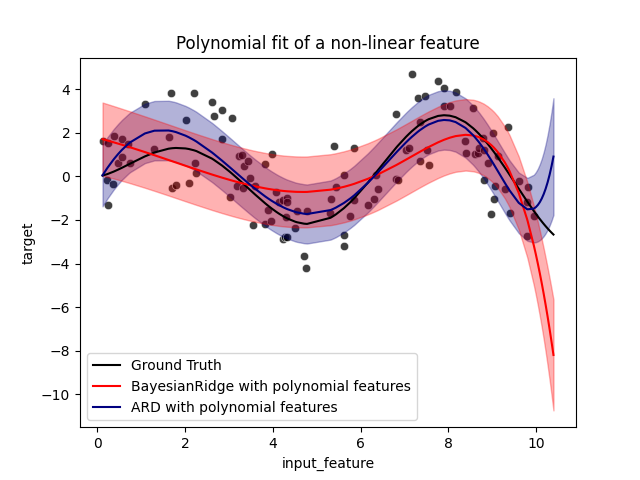
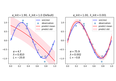
误差线代表查询点的预测高斯分布的一个标准差。请注意，当在两个模型中使用默认参数时，ARD回归能够最好地捕捉到基本事实，但进一步减少了 lambda_init 贝叶斯岭的超参数可以减少其偏差（参见示例利用Bayesian Ridge回归进行曲线匹配 ).最后，由于多元回归的固有局限性，两个模型在外推时都会失败。

Total running time of the script: （0分0.840秒）