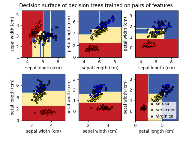
绘制在虹膜数据集上训练的决策树的决策面

绘制根据虹膜数据集的特征对训练的决策树的决策面。

看到 decision tree 有关估计器的更多信息。

对于每对虹膜特征，决策树学习由从训练样本推断出的简单阈值规则组合组成的决策边界。

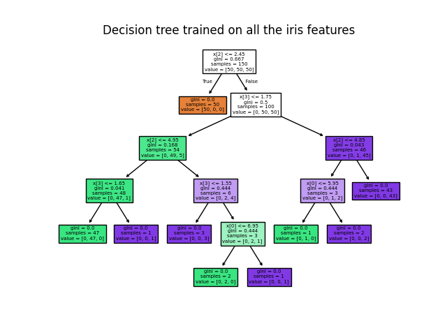
我们还展示了基于所有特征构建的模型的树结构。

# Authors: The scikit-learn developers
# SPDX-License-Identifier: BSD-3-Clause

首先加载scikit-learn随附的Iris数据集副本：

from sklearn.datasets import load_iris

iris = load_iris()

显示在所有特征对上训练的树的决策函数。

import matplotlib.pyplot as plt
import numpy as np

from sklearn.datasets import load_iris
from sklearn.inspection import DecisionBoundaryDisplay
from sklearn.tree import DecisionTreeClassifier

# Parameters
n_classes = 3
plot_colors = "ryb"
plot_step = 0.02


for pairidx, pair in enumerate([[0, 1], [0, 2], [0, 3], [1, 2], [1, 3], [2, 3]]):
    # We only take the two corresponding features
    X = iris.data[:, pair]
    y = iris.target

    # Train
    clf = DecisionTreeClassifier().fit(X, y)

    # Plot the decision boundary
    ax = plt.subplot(2, 3, pairidx + 1)
    plt.tight_layout(h_pad=0.5, w_pad=0.5, pad=2.5)
    DecisionBoundaryDisplay.from_estimator(
        clf,
        X,
        cmap=plt.cm.RdYlBu,
        response_method="predict",
        ax=ax,
        xlabel=iris.feature_names[pair[0]],
        ylabel=iris.feature_names[pair[1]],
    )

    # Plot the training points
    for i, color in zip(range(n_classes), plot_colors):
        idx = np.asarray(y == i).nonzero()
        plt.scatter(
            X[idx, 0],
            X[idx, 1],
            c=color,
            label=iris.target_names[i],
            edgecolor="black",
            s=15,
        )

plt.suptitle("Decision surface of decision trees trained on pairs of features")
plt.legend(loc="lower right", borderpad=0, handletextpad=0)
_ = plt.axis("tight")

显示对所有特征一起训练的单个决策树的结构。

from sklearn.tree import plot_tree

plt.figure()
clf = DecisionTreeClassifier().fit(iris.data, iris.target)
plot_tree(clf, filled=True)
plt.title("Decision tree trained on all the iris features")
plt.show()

相关实例

在iris数据集上绘制多类新元

Plot multi-class SGD on the iris dataset

Iris数据集的主成分分析（PCA）

Principal Component Analysis (PCA) on Iris Dataset

在虹膜数据集中绘制树木集合的决策面

Plot the decision surfaces of ensembles of trees on the iris dataset

两级AdaBoost

Two-class AdaBoost