多项和样条插值#

此示例演示如何用多个次数的多项逼近函数 degree 通过使用岭回归。我们展示了两种不同的方式 n_samples 1d点 x_i :

PolynomialFeatures 生成所有单式 degree .这给了我们所谓的范德蒙矩阵， n_samples 行和 degree + 1 列：：
```
[[1, x_0, x_0 ** 2, x_0 ** 3, ..., x_0 ** degree],
 [1, x_1, x_1 ** 2, x_1 ** 3, ..., x_1 ** degree],
 ...]
```
直观地说，这个矩阵可以被解释为伪特征（提升到一定程度的点）的矩阵。该矩阵类似于（但不同于）由多项核诱导的矩阵。
SplineTransformer 生成B样条基函数。B样条的基函数是次数的分段多项函数 degree 仅在之间非零 degree+1 连续的结。给定 n_knots 结的数量，这导致矩阵 n_samples 行和 n_knots + degree - 1 列：：
```
[[basis_1(x_0), basis_2(x_0), ...],
 [basis_1(x_1), basis_2(x_1), ...],
 ...]
```

此示例表明，这两个变压器非常适合通过线性模型对非线性效应进行建模，并使用管道添加非线性特征。核方法扩展了这一想法，可以引入非常高（甚至无限）维度的特征空间。

# Authors: The scikit-learn developers
# SPDX-License-Identifier: BSD-3-Clause

import matplotlib.pyplot as plt
import numpy as np

from sklearn.linear_model import Ridge
from sklearn.pipeline import make_pipeline
from sklearn.preprocessing import PolynomialFeatures, SplineTransformer

我们首先定义一个我们打算逼近的函数并准备绘制它。

def f(x):
    """Function to be approximated by polynomial interpolation."""
    return x * np.sin(x)


# whole range we want to plot
x_plot = np.linspace(-1, 11, 100)

为了让它有趣，我们只给出一小部分点来训练。

x_train = np.linspace(0, 10, 100)
rng = np.random.RandomState(0)
x_train = np.sort(rng.choice(x_train, size=20, replace=False))
y_train = f(x_train)

# create 2D-array versions of these arrays to feed to transformers
X_train = x_train[:, np.newaxis]
X_plot = x_plot[:, np.newaxis]

现在我们已经准备好创建多项特征和样条线，适应训练点并展示它们的内插效果。

# plot function
lw = 2
fig, ax = plt.subplots()
ax.set_prop_cycle(
    color=["black", "teal", "yellowgreen", "gold", "darkorange", "tomato"]
)
ax.plot(x_plot, f(x_plot), linewidth=lw, label="ground truth")

# plot training points
ax.scatter(x_train, y_train, label="training points")

# polynomial features
for degree in [3, 4, 5]:
    model = make_pipeline(PolynomialFeatures(degree), Ridge(alpha=1e-3))
    model.fit(X_train, y_train)
    y_plot = model.predict(X_plot)
    ax.plot(x_plot, y_plot, label=f"degree {degree}")

# B-spline with 4 + 3 - 1 = 6 basis functions
model = make_pipeline(SplineTransformer(n_knots=4, degree=3), Ridge(alpha=1e-3))
model.fit(X_train, y_train)

y_plot = model.predict(X_plot)
ax.plot(x_plot, y_plot, label="B-spline")
ax.legend(loc="lower center")
ax.set_ylim(-20, 10)
plt.show()

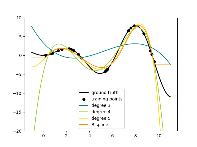
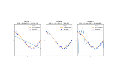
这很好地表明，更高次数的多项项可以更好地适应数据。但与此同时，过高的功率可能会表现出不必要的振荡行为，并且对于超出匹配数据范围的外推尤其危险。这是B样条的优点。它们通常适合数据和方程，并表现出非常好和平滑的行为。他们还有很好的选择来控制外推，外推默认以一个常数继续。请注意，大多数情况下，您宁愿增加结的数量，但保留 degree=3 .

为了更深入地了解生成的特征库，我们分别绘制了两个变形器的所有列。

fig, axes = plt.subplots(ncols=2, figsize=(16, 5))
pft = PolynomialFeatures(degree=3).fit(X_train)
axes[0].plot(x_plot, pft.transform(X_plot))
axes[0].legend(axes[0].lines, [f"degree {n}" for n in range(4)])
axes[0].set_title("PolynomialFeatures")

splt = SplineTransformer(n_knots=4, degree=3).fit(X_train)
axes[1].plot(x_plot, splt.transform(X_plot))
axes[1].legend(axes[1].lines, [f"spline {n}" for n in range(6)])
axes[1].set_title("SplineTransformer")

# plot knots of spline
knots = splt.bsplines_[0].t
axes[1].vlines(knots[3:-3], ymin=0, ymax=0.8, linestyles="dashed")
plt.show()

在左图中，我们识别出对应于以下简单单项式的线： x**0 到 x**3 .在右图中，我们看到六个B样条基函数， degree=3 以及期间选择的四个结位置 fit .注意有 degree 适合间隔左侧和右侧的额外结数。这些是出于技术原因而存在的，因此我们避免展示它们。每个基本函数都有局部支持，并在适合范围之外作为一个常数继续存在。这种推断行为可能会因论点而改变 extrapolation .

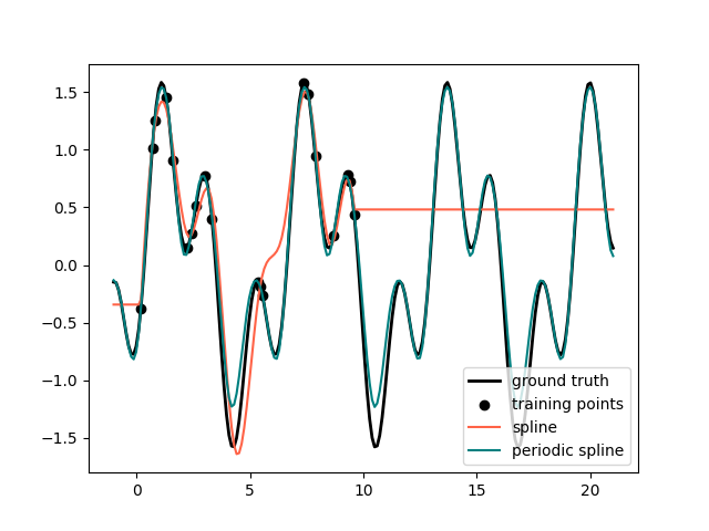
周期样条#

在之前的例子中，我们看到了在训练观察范围之外外推的多项和样条的局限性。在某些情况下，例如在季节性影响下，我们预计潜在信号会定期持续。此类效应可以使用周期样条来建模，周期样条在第一个和最后一个结处具有相等的函数值和相等的导子。在下面的情况下，我们展示了周期性的额外信息，周期样条如何在训练数据范围内和范围外提供更好的匹配。样条线周期是第一个结和最后一个结之间的距离，我们手动指定该距离。

周期样条线对于自然周期特征（例如一年中的哪一天）也很有用，因为边界结处的平滑度可以防止转换值的跳跃（例如从12月31日到1月1日）。对于此类自然周期特征或周期已知的更一般的特征，建议将此信息明确传递给 SplineTransformer 通过手动设置结。

def g(x):
    """Function to be approximated by periodic spline interpolation."""
    return np.sin(x) - 0.7 * np.cos(x * 3)


y_train = g(x_train)

# Extend the test data into the future:
x_plot_ext = np.linspace(-1, 21, 200)
X_plot_ext = x_plot_ext[:, np.newaxis]

lw = 2
fig, ax = plt.subplots()
ax.set_prop_cycle(color=["black", "tomato", "teal"])
ax.plot(x_plot_ext, g(x_plot_ext), linewidth=lw, label="ground truth")
ax.scatter(x_train, y_train, label="training points")

for transformer, label in [
    (SplineTransformer(degree=3, n_knots=10), "spline"),
    (
        SplineTransformer(
            degree=3,
            knots=np.linspace(0, 2 * np.pi, 10)[:, None],
            extrapolation="periodic",
        ),
        "periodic spline",
    ),
]:
    model = make_pipeline(transformer, Ridge(alpha=1e-3))
    model.fit(X_train, y_train)
    y_plot_ext = model.predict(X_plot_ext)
    ax.plot(x_plot_ext, y_plot_ext, label=label)

ax.legend()
fig.show()

fig, ax = plt.subplots()
knots = np.linspace(0, 2 * np.pi, 4)
splt = SplineTransformer(knots=knots[:, None], degree=3, extrapolation="periodic").fit(
    X_train
)
ax.plot(x_plot_ext, splt.transform(X_plot_ext))
ax.legend(ax.lines, [f"spline {n}" for n in range(3)])
plt.show()

Total running time of the script: （0分0.340秒）