模型正规化对训练和测试误差的影响#

在这个例子中，我们评估了线性模型中正规化参数的影响，称为 ElasticNet .为了执行此评估，我们使用验证曲线， ValidationCurveDisplay .该曲线显示了模型对于不同的正规化参数值的训练和测试分数。

一旦我们识别出最佳正规化参数，我们就会比较模型的真实系数和估计系数，以确定模型是否能够从有噪的输入数据中恢复系数。

# Authors: The scikit-learn developers
# SPDX-License-Identifier: BSD-3-Clause

生成示例数据#

我们生成一个回归数据集，其中包含许多相对于样本数量的特征。然而，只有10%的功能具有信息性。在这种情况下，暴露L1惩罚的线性模型通常用于恢复稀疏系数集。

from sklearn.datasets import make_regression
from sklearn.model_selection import train_test_split

n_samples_train, n_samples_test, n_features = 150, 300, 500
X, y, true_coef = make_regression(
    n_samples=n_samples_train + n_samples_test,
    n_features=n_features,
    n_informative=50,
    shuffle=False,
    noise=1.0,
    coef=True,
    random_state=42,
)
X_train, X_test, y_train, y_test = train_test_split(
    X, y, train_size=n_samples_train, test_size=n_samples_test, shuffle=False
)

模型定义#

在这里，我们不使用仅暴露L1罚分的模型。相反，我们使用 ElasticNet 暴露L1和L2处罚的模型。

我们修复 l1_ratio 参数，以便模型找到的解仍然稀疏。因此，这种类型的模型试图找到稀疏解，但同时也试图将所有系数缩小到零。

此外，我们强制模型的系数为正，因为我们知道 make_regression 产生具有正信号的响应。因此我们使用这个预先知识来获得更好的模型。

from sklearn.linear_model import ElasticNet

enet = ElasticNet(l1_ratio=0.9, positive=True, max_iter=10_000)

评估正规化参数的影响#

为了评估正规化参数的影响，我们使用验证曲线。该曲线显示了模型对于不同的正规化参数值的训练和测试分数。

正则化 alpha 是应用于模型系数的参数：当它趋于零时，不应用正规化，模型尝试以最小的误差来适应训练数据。然而，当特征有噪音时，它会导致过度匹配。当 alpha 增加时，模型系数就会受到约束，因此模型无法如此接近地匹配训练数据，从而避免过度匹配。然而，如果应用了太多的正规化，模型将不适合数据并且无法正确捕获信号。

验证曲线有助于在两个极端之间找到一个很好的折衷：模型没有正则化，因此足够灵活以拟合信号，但又不太灵活而不能过度拟合。的 ValidationCurveDisplay 允许我们显示一系列alpha值的训练和验证分数。

import numpy as np

from sklearn.model_selection import ValidationCurveDisplay

alphas = np.logspace(-5, 1, 60)
disp = ValidationCurveDisplay.from_estimator(
    enet,
    X_train,
    y_train,
    param_name="alpha",
    param_range=alphas,
    scoring="r2",
    n_jobs=2,
    score_type="both",
)
disp.ax_.set(
    title=r"Validation Curve for ElasticNet (R$^2$ Score)",
    xlabel=r"alpha (regularization strength)",
    ylabel="R$^2$ Score",
)

test_scores_mean = disp.test_scores.mean(axis=1)
idx_avg_max_test_score = np.argmax(test_scores_mean)
disp.ax_.vlines(
    alphas[idx_avg_max_test_score],
    disp.ax_.get_ylim()[0],
    test_scores_mean[idx_avg_max_test_score],
    color="k",
    linewidth=2,
    linestyle="--",
    label=f"Optimum on test\n$\\alpha$ = {alphas[idx_avg_max_test_score]:.2e}",
)
_ = disp.ax_.legend(loc="lower right")

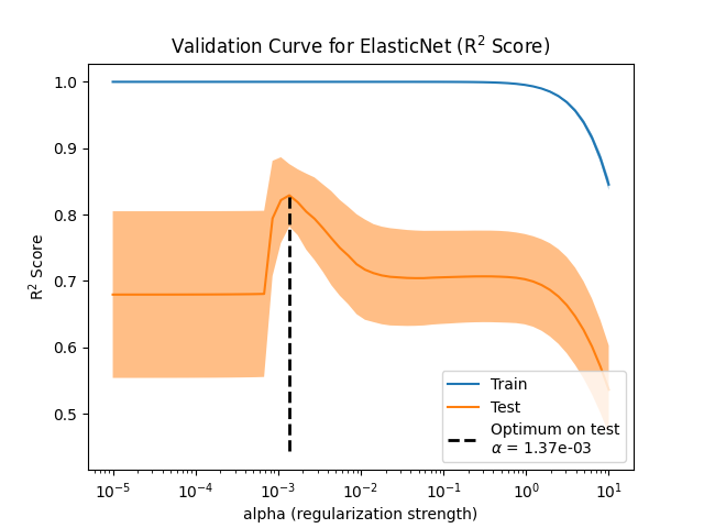
Validation Curve for ElasticNet (R$^2$ Score)

为了找到最佳正规化参数，我们可以选择 alpha 这最大化了验证分数。

系数比较#

既然我们已经确定了最佳正规化参数，我们就可以比较真实系数和估计系数了。

首先，让我们将正规化参数设置为最佳值，并将模型与训练数据匹配。此外，我们还将显示该模型的测试分数。

enet.set_params(alpha=alphas[idx_avg_max_test_score]).fit(X_train, y_train)
print(
    f"Test score: {enet.score(X_test, y_test):.3f}",
)

Test score: 0.884

现在，我们绘制真实系数和估计系数。

import matplotlib.pyplot as plt

fig, axs = plt.subplots(ncols=2, figsize=(12, 6), sharex=True, sharey=True)
for ax, coef, title in zip(axs, [true_coef, enet.coef_], ["True", "Model"]):
    ax.stem(coef)
    ax.set(
        title=f"{title} Coefficients",
        xlabel="Feature Index",
        ylabel="Coefficient Value",
    )
fig.suptitle(
    "Comparison of the coefficients of the true generative model and \n"
    "the estimated elastic net coefficients"
)

plt.show()

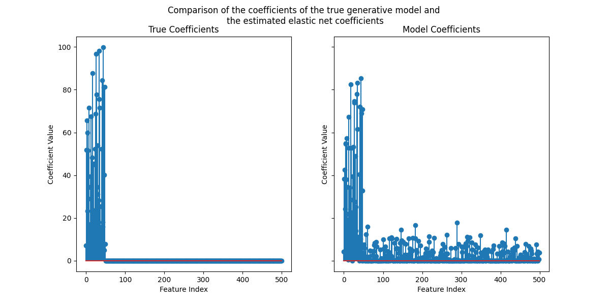
Comparison of the coefficients of the true generative model and the estimated elastic net coefficients, True Coefficients, Model Coefficients

虽然原始系数是稀疏的，但估计的系数并不那么稀疏。原因是我们修复了 l1_ratio 参数为0.9。我们可以通过增加 l1_ratio 参数.

然而，我们观察到，对于真实生成模型中接近零的估计系数，我们的模型会将它们缩小为零。因此，我们不会恢复真实系数，但我们会得到与测试集中获得的性能一致的合理结果。

Total running time of the script: （0分6.770秒）