具有不同支持机核的地块分类边界

这个例子展示了 SVC （支持向量分类器）影响二元、二维分类问题中的分类边界。

SVCs的目标是找到一个超平面，通过最大化每个类别最外面的数据点之间的裕度来有效地分离训练数据中的类别。这是通过找到最佳权重载体来实现的 \(w\) 它定义了决策边界超平面，并最大限度地减少了错误分类样本的铰链损失总和，由 hinge_loss 功能默认情况下，使用参数应用规则化 C=1 ，这允许一定程度的误分类容忍度。

如果数据在原始特征空间中不可线性分离，则可以设置非线性核参数。根据内核的不同，该过程涉及添加新功能或转换现有功能以丰富数据并可能为数据添加意义。当除了 "linear" is set, the SVC applies the kernel trick ，它使用核函数计算数据点对之间的相似性，而无需显式转换整个数据集。核技巧通过仅考虑所有数据点对之间的关系来超越整个数据集否则必要的矩阵变换。核函数使用点积将两个载体（每对观察）映射到它们的相似性。

然后可以使用核函数计算超平面，就像数据集在更高维度的空间中表示一样。使用核函数而不是显式矩阵变换可以提高性能，因为核函数的时间复杂度为 \(O({n}^2)\) ，而矩阵变换根据所应用的特定变换进行缩放。

在这个例子中，我们比较了支持向量机最常见的内核类型：线性内核 ("linear" ），多项核 ("poly" ），辐射基函数核 ("rbf" ）和Sigmoid内核 ("sigmoid" ).

# Authors: The scikit-learn developers
# SPDX-License-Identifier: BSD-3-Clause

创建数据集

我们创建一个包含16个样本和两个类别的二维分类数据集。我们用与各自目标相匹配的颜色绘制样本。

import matplotlib.pyplot as plt
import numpy as np

X = np.array(
    [
        [0.4, -0.7],
        [-1.5, -1.0],
        [-1.4, -0.9],
        [-1.3, -1.2],
        [-1.1, -0.2],
        [-1.2, -0.4],
        [-0.5, 1.2],
        [-1.5, 2.1],
        [1.0, 1.0],
        [1.3, 0.8],
        [1.2, 0.5],
        [0.2, -2.0],
        [0.5, -2.4],
        [0.2, -2.3],
        [0.0, -2.7],
        [1.3, 2.1],
    ]
)

y = np.array([0, 0, 0, 0, 0, 0, 0, 0, 1, 1, 1, 1, 1, 1, 1, 1])

# Plotting settings
fig, ax = plt.subplots(figsize=(4, 3))
x_min, x_max, y_min, y_max = -3, 3, -3, 3
ax.set(xlim=(x_min, x_max), ylim=(y_min, y_max))

# Plot samples by color and add legend
scatter = ax.scatter(X[:, 0], X[:, 1], s=150, c=y, label=y, edgecolors="k")
ax.legend(*scatter.legend_elements(), loc="upper right", title="Classes")
ax.set_title("Samples in two-dimensional feature space")
_ = plt.show()

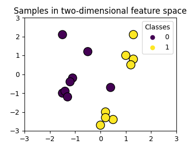
我们可以看到样本并不能通过直线明显分开。

训练SV模型并绘制决策边界

我们定义一个适合 SVC 分类器，允许 kernel 参数作为输入，然后使用绘制模型学习的决策边界 DecisionBoundaryDisplay .

Notice that for the sake of simplicity, the C parameter is set to its default value (C=1) in this example and the gamma parameter is set to gamma=2 across all kernels, although it is automatically ignored for the linear kernel. In a real classification task, where performance matters, parameter tuning (by using GridSearchCV for instance) is highly recommended to capture different structures within the data.

设置 response_method="predict" 在 DecisionBoundaryDisplay 根据预测的类别为区域着色。使用 response_method="decision_function" 允许我们绘制决策边界及其两侧的裕度。最后，通过 support_vectors_ 训练的SV的属性，并绘制。

from sklearn import svm
from sklearn.inspection import DecisionBoundaryDisplay


def plot_training_data_with_decision_boundary(
    kernel, ax=None, long_title=True, support_vectors=True
):
    # Train the SVC
    clf = svm.SVC(kernel=kernel, gamma=2).fit(X, y)

    # Settings for plotting
    if ax is None:
        _, ax = plt.subplots(figsize=(4, 3))
    x_min, x_max, y_min, y_max = -3, 3, -3, 3
    ax.set(xlim=(x_min, x_max), ylim=(y_min, y_max))

    # Plot decision boundary and margins
    common_params = {"estimator": clf, "X": X, "ax": ax}
    DecisionBoundaryDisplay.from_estimator(
        **common_params,
        response_method="predict",
        plot_method="pcolormesh",
        alpha=0.3,
    )
    DecisionBoundaryDisplay.from_estimator(
        **common_params,
        response_method="decision_function",
        plot_method="contour",
        levels=[-1, 0, 1],
        colors=["k", "k", "k"],
        linestyles=["--", "-", "--"],
    )

    if support_vectors:
        # Plot bigger circles around samples that serve as support vectors
        ax.scatter(
            clf.support_vectors_[:, 0],
            clf.support_vectors_[:, 1],
            s=150,
            facecolors="none",
            edgecolors="k",
        )

    # Plot samples by color and add legend
    ax.scatter(X[:, 0], X[:, 1], c=y, s=30, edgecolors="k")
    ax.legend(*scatter.legend_elements(), loc="upper right", title="Classes")
    if long_title:
        ax.set_title(f" Decision boundaries of {kernel} kernel in SVC")
    else:
        ax.set_title(kernel)

    if ax is None:
        plt.show()

线性核

线性核是输入样本的点积：

\[K(\mathbf{x}_1, \mathbf{x}_2) = \mathbf{x}_1^\top \mathbf{x}_2\]

It is then applied to any combination of two data points (samples) in the dataset. The dot product of the two points determines the cosine_similarity between both points. The higher the value, the more similar the points are.

plot_training_data_with_decision_boundary("linear")

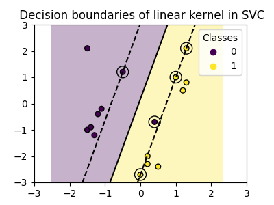
训练 SVC 在线性核上产生未变换的特征空间，其中超平面和边缘是直线。由于线性核缺乏表达性，训练的类不能完美地捕获训练数据。

多项式核

多项核改变了相似性的概念。内核函数定义为：

\[K(\mathbf{x}_1, \mathbf{x}_2) = (\gamma \cdot \ \mathbf{x}_1^\top\mathbf{x}_2 + r)^d\]

where \({d}\) is the degree (degree) of the polynomial, \({\gamma}\) (gamma) controls the influence of each individual training sample on the decision boundary and \({r}\) is the bias term (coef0) that shifts the data up or down. Here, we use the default value for the degree of the polynomial in the kernel function (degree=3). When coef0=0 (the default), the data is only transformed, but no additional dimension is added. Using a polynomial kernel is equivalent to creating PolynomialFeatures and then fitting a SVC with a linear kernel on the transformed data, although this alternative approach would be computationally expensive for most datasets.

plot_training_data_with_decision_boundary("poly")

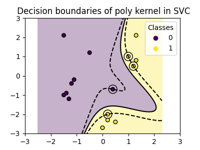
具有的多项核 gamma=2 很好地适应训练数据，导致超平面两侧的边缘相应弯曲。

RBF核

The radial basis function (RBF) kernel, also known as the Gaussian kernel, is the default kernel for Support Vector Machines in scikit-learn. It measures similarity between two data points in infinite dimensions and then approaches classification by majority vote. The kernel function is defined as:

\[K(\mathbf{x}_1, \mathbf{x}_2) = \exp\left(-\gamma \cdot {\|\mathbf{x}_1 - \mathbf{x}_2\|^2}\right)\]

where \({\gamma}\) (gamma) controls the influence of each individual training sample on the decision boundary.

The larger the euclidean distance between two points \(\|\mathbf{x}_1 - \mathbf{x}_2\|^2\) the closer the kernel function is to zero. This means that two points far away are more likely to be dissimilar.

plot_training_data_with_decision_boundary("rbf")

在图中，我们可以看到决策边界如何倾向于围绕彼此接近的数据点收缩。

Sigmoid核

sigmoid内核函数定义为：

\[K(\mathbf{x}_1, \mathbf{x}_2) = \tanh(\gamma \cdot \mathbf{x}_1^\top\mathbf{x}_2 + r)\]

where the kernel coefficient \({\gamma}\) (gamma) controls the influence of each individual training sample on the decision boundary and \({r}\) is the bias term (coef0) that shifts the data up or down.

在Sigmoid核中，使用双曲切函数计算两个数据点之间的相似度 (\(\tanh\) ).核函数缩放并可能移动两点的点积 (\(\mathbf{x}_1\) 和 \(\mathbf{x}_2\) ).

plot_training_data_with_decision_boundary("sigmoid")

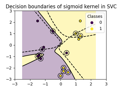
我们可以看到，使用sigmoid内核获得的决策边界看起来弯曲且不规则。决策边界试图通过拟合S形曲线来分离类别，从而导致可能无法很好地推广到未知数据的复杂边界。从这个例子中可以明显看出，sigmoid内核在处理呈现sigmoid形状的数据时有非常特定的用例。在这个例子中，仔细的微调可能会发现更通用的决策边界。由于其特殊性，与其他内核相比，sigmoid内核在实践中不太常用。

结论

在这个例子中，我们可视化了用提供的数据集训练的决策边界。这些图直观地展示了不同的内核如何利用训练数据来确定分类边界。

超平面和边缘虽然是间接计算的，但可以想象为转换后的特征空间中的平面。然而，在图中，它们是相对于原始特征空间来表示的，从而导致多项核、RBS和Sigmoid核的曲线决策边界。

请注意，这些图不会评估单个籽粒的准确性或质量。它们旨在提供对不同内核如何使用训练数据的视觉理解。

为了全面评估，微调 SVC 参数使用技术，如 GridSearchCV 建议捕获数据中的基础结构。

异或数据集

非线性可分的数据集的一个经典示例是异或模式。在这里，我们演示了不同的内核如何在这样的数据集上工作。

xx, yy = np.meshgrid(np.linspace(-3, 3, 500), np.linspace(-3, 3, 500))
np.random.seed(0)
X = np.random.randn(300, 2)
y = np.logical_xor(X[:, 0] > 0, X[:, 1] > 0)

_, ax = plt.subplots(2, 2, figsize=(8, 8))
args = dict(long_title=False, support_vectors=False)
plot_training_data_with_decision_boundary("linear", ax[0, 0], **args)
plot_training_data_with_decision_boundary("poly", ax[0, 1], **args)
plot_training_data_with_decision_boundary("rbf", ax[1, 0], **args)
plot_training_data_with_decision_boundary("sigmoid", ax[1, 1], **args)
plt.show()

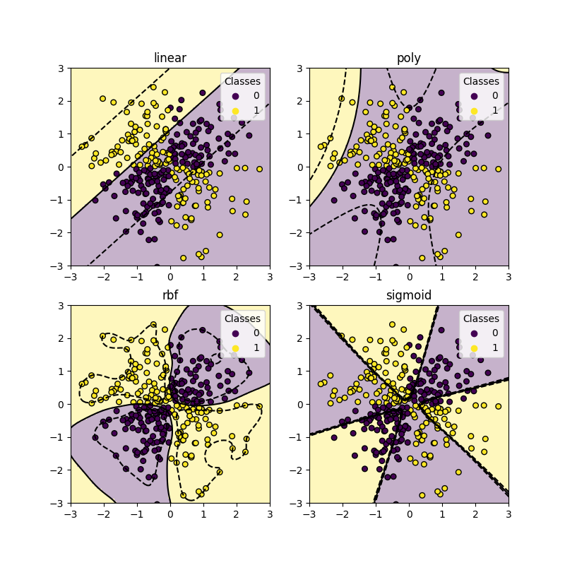
正如您从上面的图中可以看到的，只有 rbf 内核可以为上述数据集找到合理的决策边界。

相关实例

RBF SVM参数

RBF SVM parameters

在虹膜数据集中绘制不同的支持者分类器

Plot different SVM classifiers in the iris dataset

Iris数据集上半监督分类器与支持机的决策边界

Decision boundary of semi-supervised classifiers versus SVM on the Iris dataset

两级AdaBoost

Two-class AdaBoost