将数据映射到正态分布

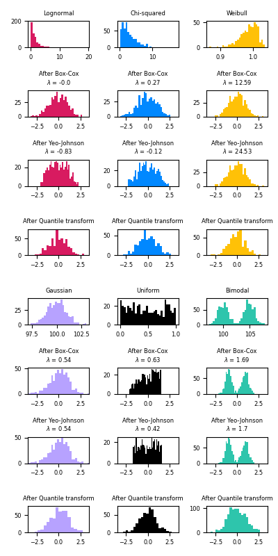
此示例演示了Box-Cox和Yeo-Johnson变换的使用，通过 PowerTransformer 将数据从各种分布映射到正态分布。

功率变换作为需要同方差和正态性的建模问题的变换非常有用。以下是应用于六种不同概率分布的Box-Cox和Yeo-Johnwon的示例：对正态、卡方、威布尔、高斯、均匀和双峰。

请注意，当应用于某些数据集时，转换成功地将数据映射到正态分布，但对其他数据集无效。这凸显了转换前后可视化数据的重要性。

另请注意，尽管Box-Cox在log正态和卡方分布方面似乎比Yeo-Johnson表现更好，但请记住Box-Cox不支持负值的输入。

为了进行比较，我们还添加了来自 QuantileTransformer .只要有足够的训练样本（数千个），它可以将任何任意分布强制为高斯分布。由于它是一种非参数方法，因此它比参数方法（Box-Cox和Yeo-Johnson）更难解释。

在“小”数据集（少于几百个点）上，分位数Transformer容易过拟合。然后建议使用电力变压器。

# Authors: The scikit-learn developers
# SPDX-License-Identifier: BSD-3-Clause

import matplotlib.pyplot as plt
import numpy as np

from sklearn.model_selection import train_test_split
from sklearn.preprocessing import PowerTransformer, QuantileTransformer

N_SAMPLES = 1000
FONT_SIZE = 6
BINS = 30


rng = np.random.RandomState(304)
bc = PowerTransformer(method="box-cox")
yj = PowerTransformer(method="yeo-johnson")
# n_quantiles is set to the training set size rather than the default value
# to avoid a warning being raised by this example
qt = QuantileTransformer(
    n_quantiles=500, output_distribution="normal", random_state=rng
)
size = (N_SAMPLES, 1)


# lognormal distribution
X_lognormal = rng.lognormal(size=size)

# chi-squared distribution
df = 3
X_chisq = rng.chisquare(df=df, size=size)

# weibull distribution
a = 50
X_weibull = rng.weibull(a=a, size=size)

# gaussian distribution
loc = 100
X_gaussian = rng.normal(loc=loc, size=size)

# uniform distribution
X_uniform = rng.uniform(low=0, high=1, size=size)

# bimodal distribution
loc_a, loc_b = 100, 105
X_a, X_b = rng.normal(loc=loc_a, size=size), rng.normal(loc=loc_b, size=size)
X_bimodal = np.concatenate([X_a, X_b], axis=0)


# create plots
distributions = [
    ("Lognormal", X_lognormal),
    ("Chi-squared", X_chisq),
    ("Weibull", X_weibull),
    ("Gaussian", X_gaussian),
    ("Uniform", X_uniform),
    ("Bimodal", X_bimodal),
]

colors = ["#D81B60", "#0188FF", "#FFC107", "#B7A2FF", "#000000", "#2EC5AC"]

fig, axes = plt.subplots(nrows=8, ncols=3, figsize=plt.figaspect(2))
axes = axes.flatten()
axes_idxs = [
    (0, 3, 6, 9),
    (1, 4, 7, 10),
    (2, 5, 8, 11),
    (12, 15, 18, 21),
    (13, 16, 19, 22),
    (14, 17, 20, 23),
]
axes_list = [(axes[i], axes[j], axes[k], axes[l]) for (i, j, k, l) in axes_idxs]


for distribution, color, axes in zip(distributions, colors, axes_list):
    name, X = distribution
    X_train, X_test = train_test_split(X, test_size=0.5)

    # perform power transforms and quantile transform
    X_trans_bc = bc.fit(X_train).transform(X_test)
    lmbda_bc = round(bc.lambdas_[0], 2)
    X_trans_yj = yj.fit(X_train).transform(X_test)
    lmbda_yj = round(yj.lambdas_[0], 2)
    X_trans_qt = qt.fit(X_train).transform(X_test)

    ax_original, ax_bc, ax_yj, ax_qt = axes

    ax_original.hist(X_train, color=color, bins=BINS)
    ax_original.set_title(name, fontsize=FONT_SIZE)
    ax_original.tick_params(axis="both", which="major", labelsize=FONT_SIZE)

    for ax, X_trans, meth_name, lmbda in zip(
        (ax_bc, ax_yj, ax_qt),
        (X_trans_bc, X_trans_yj, X_trans_qt),
        ("Box-Cox", "Yeo-Johnson", "Quantile transform"),
        (lmbda_bc, lmbda_yj, None),
    ):
        ax.hist(X_trans, color=color, bins=BINS)
        title = "After {}".format(meth_name)
        if lmbda is not None:
            title += "\n$\\lambda$ = {}".format(lmbda)
        ax.set_title(title, fontsize=FONT_SIZE)
        ax.tick_params(axis="both", which="major", labelsize=FONT_SIZE)
        ax.set_xlim([-3.5, 3.5])


plt.tight_layout()
plt.show()

相关实例

比较不同缩放器对数据的影响与离群值

Compare the effect of different scalers on data with outliers

Gradient Boosting中的提前停止

Early stopping in Gradient Boosting

缩放SVCs的正规化参数

Scaling the regularization parameter for SVCs

随机投影嵌入的Johnson-Lindenstrauss界

The Johnson-Lindenstrauss bound for embedding with random projections