了解决策树结构#

可以分析决策树结构，以进一步了解特征与要预测的目标之间的关系。在这个例子中，我们展示了如何检索：

the binary tree structure;
每个节点的深度以及它是否是叶子;
样本使用 decision_path 方法;
使用应用方法获得的样本到达的叶子;
用于预测样本的规则;
一组样本共享的决策路径。

# Authors: The scikit-learn developers
# SPDX-License-Identifier: BSD-3-Clause

import numpy as np
from matplotlib import pyplot as plt

from sklearn import tree
from sklearn.datasets import load_iris
from sklearn.model_selection import train_test_split
from sklearn.tree import DecisionTreeClassifier

训练树分类器#

首先，我们适合 DecisionTreeClassifier 使用 load_iris 数据集。

iris = load_iris()
X = iris.data
y = iris.target
X_train, X_test, y_train, y_test = train_test_split(X, y, random_state=0)

clf = DecisionTreeClassifier(max_leaf_nodes=3, random_state=0)
clf.fit(X_train, y_train)

DecisionTreeClassifier(max_leaf_nodes=3, random_state=0)

In a Jupyter environment, please rerun this cell to show the HTML representation or trust the notebook.
On GitHub, the HTML representation is unable to render, please try loading this page with nbviewer.org.

树结构#

决策分类器有一个名为 tree_ 这允许访问低级属性，例如 node_count 、节点总数，以及 max_depth ，树的最大深度。的 tree_.compute_node_depths() 方法计算树中每个节点的深度。 tree_ 还存储整个二元树结构，表示为多个并行阵列。每个数组的第i个元素保存有关节点的信息 i .节点0是树的根。某些数组仅适用于叶子或分裂节点。在这种情况下，其他类型的节点的值是任意的。例如，数组 feature 和 threshold 仅适用于分裂节点。因此，这些数组中叶节点的值是任意的。

在这些阵列中，我们有：

children_left[i] ：节点左子节点的id i 如果是叶节点，则为-1
children_right[i] ：节点右子节点的id i 如果是叶节点，则为-1
feature[i] ：用于拆分节点的功能 i
threshold[i] ：节点阈值 i
n_node_samples[i] ：到达节点的训练样本数 i
impurity[i] ：节点处的杂质 i
weighted_n_node_samples[i] ：到达节点的训练样本加权数 i
value[i, j, k] ：到达输出j和类k的节点i的训练样本的摘要（对于回归树，类设置为1）。请参阅下文以了解有关 value .

使用数组，我们可以遍历树结构来计算各种属性。下面，我们将计算每个节点的深度以及它是否是叶子。

n_nodes = clf.tree_.node_count
children_left = clf.tree_.children_left
children_right = clf.tree_.children_right
feature = clf.tree_.feature
threshold = clf.tree_.threshold
values = clf.tree_.value

node_depth = np.zeros(shape=n_nodes, dtype=np.int64)
is_leaves = np.zeros(shape=n_nodes, dtype=bool)
stack = [(0, 0)]  # start with the root node id (0) and its depth (0)
while len(stack) > 0:
    # `pop` ensures each node is only visited once
    node_id, depth = stack.pop()
    node_depth[node_id] = depth

    # If the left and right child of a node is not the same we have a split
    # node
    is_split_node = children_left[node_id] != children_right[node_id]
    # If a split node, append left and right children and depth to `stack`
    # so we can loop through them
    if is_split_node:
        stack.append((children_left[node_id], depth + 1))
        stack.append((children_right[node_id], depth + 1))
    else:
        is_leaves[node_id] = True

print(
    "The binary tree structure has {n} nodes and has "
    "the following tree structure:\n".format(n=n_nodes)
)
for i in range(n_nodes):
    if is_leaves[i]:
        print(
            "{space}node={node} is a leaf node with value={value}.".format(
                space=node_depth[i] * "\t", node=i, value=np.around(values[i], 3)
            )
        )
    else:
        print(
            "{space}node={node} is a split node with value={value}: "
            "go to node {left} if X[:, {feature}] <= {threshold} "
            "else to node {right}.".format(
                space=node_depth[i] * "\t",
                node=i,
                left=children_left[i],
                feature=feature[i],
                threshold=threshold[i],
                right=children_right[i],
                value=np.around(values[i], 3),
            )
        )

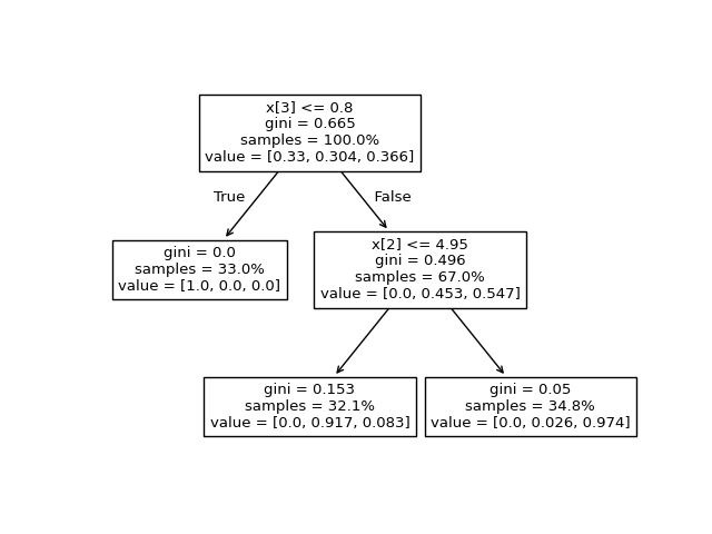
The binary tree structure has 5 nodes and has the following tree structure:

node=0 is a split node with value=[[0.33  0.304 0.366]]: go to node 1 if X[:, 3] <= 0.800000011920929 else to node 2.
        node=1 is a leaf node with value=[[1. 0. 0.]].
        node=2 is a split node with value=[[0.    0.453 0.547]]: go to node 3 if X[:, 2] <= 4.950000047683716 else to node 4.
                node=3 is a leaf node with value=[[0.    0.917 0.083]].
                node=4 is a leaf node with value=[[0.    0.026 0.974]].

这里使用的值数组是什么？#

的 tree_.value 数组是形状的3D数组 [n_nodes, n_classes, n_outputs] 它提供了到达每个类别和每个输出的节点的样本比例。每个节点具有 value 数组，这是每个输出和类到达此节点的加权样本相对于父节点的比例。

可以将其转换为到达节点的样本的绝对加权数，方法是将此数乘以 tree_.weighted_n_node_samples[node_idx] 对于给定的节点。请注意，本例中不使用样本权重，因此加权样本数是到达节点的样本数，因为默认情况下每个样本的权重为1。

例如，在上面基于iris数据集构建的树中，根节点具有 value = [0.33, 0.304, 0.366] 表明根节点处有33%的0类样本、30.4%的1类样本和36.6%的2类样本。可以通过乘以到达根节点的样本数将其转换为样本的绝对数，即 tree_.weighted_n_node_samples[0] .那么根节点有 value = [37, 34, 41] ，指示根节点处有37个类0样本、34个类1样本和41个类2样本。

穿过树，样本被分裂，结果是 value 到达每个节点的数组都会发生变化。根节点的左子节点具有 value = [1., 0, 0] （或 value = [37, 0, 0] 当转换为样本的绝对数时），因为左子节点中的所有37个样本都来自类0。

注意：在这个例子中， n_outputs=1 ，但树分类器也可以处理多输出问题。的 value 每个节点上的数组将只是一个2D数组。

我们可以将上述输出与决策树的图进行比较。在这里，我们显示到达与实际元素对应的每个节点的每个类的样本比例 tree_.value 阵

tree.plot_tree(clf, proportion=True)
plt.show()

决策轨迹#

我们还可以检索感兴趣样本的决策路径。的 decision_path 方法输出一个指示符矩阵，允许我们检索感兴趣的样本所穿过的节点。指标矩阵中位置的非零元素 (i, j) 表示样品 i 经过节点 j .或者，对于一个样本 i ，行中非零元素的位置 i 指示符矩阵的指定样本经过的节点的id。

可以使用 apply 法这将返回每个感兴趣的样本所到达的叶的节点id数组。使用叶id和 decision_path 我们可以获得用于预测一个样本或一组样本的分裂条件。首先，让我们针对一个样本进行这一操作。注意 node_index 是一个稀疏矩阵。

node_indicator = clf.decision_path(X_test)
leaf_id = clf.apply(X_test)

sample_id = 0
# obtain ids of the nodes `sample_id` goes through, i.e., row `sample_id`
node_index = node_indicator.indices[
    node_indicator.indptr[sample_id] : node_indicator.indptr[sample_id + 1]
]

print("Rules used to predict sample {id}:\n".format(id=sample_id))
for node_id in node_index:
    # continue to the next node if it is a leaf node
    if leaf_id[sample_id] == node_id:
        continue

    # check if value of the split feature for sample 0 is below threshold
    if X_test[sample_id, feature[node_id]] <= threshold[node_id]:
        threshold_sign = "<="
    else:
        threshold_sign = ">"

    print(
        "decision node {node} : (X_test[{sample}, {feature}] = {value}) "
        "{inequality} {threshold})".format(
            node=node_id,
            sample=sample_id,
            feature=feature[node_id],
            value=X_test[sample_id, feature[node_id]],
            inequality=threshold_sign,
            threshold=threshold[node_id],
        )
    )

Rules used to predict sample 0:

decision node 0 : (X_test[0, 3] = 2.4) > 0.800000011920929)
decision node 2 : (X_test[0, 2] = 5.1) > 4.950000047683716)

对于一组样本，我们可以确定样本经过的公共节点。

sample_ids = [0, 1]
# boolean array indicating the nodes both samples go through
common_nodes = node_indicator.toarray()[sample_ids].sum(axis=0) == len(sample_ids)
# obtain node ids using position in array
common_node_id = np.arange(n_nodes)[common_nodes]

print(
    "\nThe following samples {samples} share the node(s) {nodes} in the tree.".format(
        samples=sample_ids, nodes=common_node_id
    )
)
print("This is {prop}% of all nodes.".format(prop=100 * len(common_node_id) / n_nodes))

The following samples [0, 1] share the node(s) [0 2] in the tree.
This is 40.0% of all nodes.

Total running time of the script: （0分0.055秒）