股票市场结构可视化#

这个例子使用了几种无监督学习技术来从历史报价的变化中提取股票市场结构。

我们使用的数量是报价的每日变化：链接的报价往往会在一天内相互波动。

# Authors: The scikit-learn developers
# SPDX-License-Identifier: BSD-3-Clause

从互联网上删除数据#

数据为2003年至2008年。这是相当平静的：不久前，我们就有了高科技公司，而且是在2008年崩溃之前。这种历史数据可以从诸如 data.nasdaq.com 和 alphavantage.co .

import sys

import numpy as np
import pandas as pd

symbol_dict = {
    "TOT": "Total",
    "XOM": "Exxon",
    "CVX": "Chevron",
    "COP": "ConocoPhillips",
    "VLO": "Valero Energy",
    "MSFT": "Microsoft",
    "IBM": "IBM",
    "TWX": "Time Warner",
    "CMCSA": "Comcast",
    "CVC": "Cablevision",
    "YHOO": "Yahoo",
    "DELL": "Dell",
    "HPQ": "HP",
    "AMZN": "Amazon",
    "TM": "Toyota",
    "CAJ": "Canon",
    "SNE": "Sony",
    "F": "Ford",
    "HMC": "Honda",
    "NAV": "Navistar",
    "NOC": "Northrop Grumman",
    "BA": "Boeing",
    "KO": "Coca Cola",
    "MMM": "3M",
    "MCD": "McDonald's",
    "PEP": "Pepsi",
    "K": "Kellogg",
    "UN": "Unilever",
    "MAR": "Marriott",
    "PG": "Procter Gamble",
    "CL": "Colgate-Palmolive",
    "GE": "General Electrics",
    "WFC": "Wells Fargo",
    "JPM": "JPMorgan Chase",
    "AIG": "AIG",
    "AXP": "American express",
    "BAC": "Bank of America",
    "GS": "Goldman Sachs",
    "AAPL": "Apple",
    "SAP": "SAP",
    "CSCO": "Cisco",
    "TXN": "Texas Instruments",
    "XRX": "Xerox",
    "WMT": "Wal-Mart",
    "HD": "Home Depot",
    "GSK": "GlaxoSmithKline",
    "PFE": "Pfizer",
    "SNY": "Sanofi-Aventis",
    "NVS": "Novartis",
    "KMB": "Kimberly-Clark",
    "R": "Ryder",
    "GD": "General Dynamics",
    "RTN": "Raytheon",
    "CVS": "CVS",
    "CAT": "Caterpillar",
    "DD": "DuPont de Nemours",
}


symbols, names = np.array(sorted(symbol_dict.items())).T

quotes = []

for symbol in symbols:
    print("Fetching quote history for %r" % symbol, file=sys.stderr)
    url = (
        "https://raw.githubusercontent.com/scikit-learn/examples-data/"
        "master/financial-data/{}.csv"
    )
    quotes.append(pd.read_csv(url.format(symbol)))

close_prices = np.vstack([q["close"] for q in quotes])
open_prices = np.vstack([q["open"] for q in quotes])

# The daily variations of the quotes are what carry the most information
variation = close_prices - open_prices

Fetching quote history for np.str_('AAPL')
Fetching quote history for np.str_('AIG')
Fetching quote history for np.str_('AMZN')
Fetching quote history for np.str_('AXP')
Fetching quote history for np.str_('BA')
Fetching quote history for np.str_('BAC')
Fetching quote history for np.str_('CAJ')
Fetching quote history for np.str_('CAT')
Fetching quote history for np.str_('CL')
Fetching quote history for np.str_('CMCSA')
Fetching quote history for np.str_('COP')
Fetching quote history for np.str_('CSCO')
Fetching quote history for np.str_('CVC')
Fetching quote history for np.str_('CVS')
Fetching quote history for np.str_('CVX')
Fetching quote history for np.str_('DD')
Fetching quote history for np.str_('DELL')
Fetching quote history for np.str_('F')
Fetching quote history for np.str_('GD')
Fetching quote history for np.str_('GE')
Fetching quote history for np.str_('GS')
Fetching quote history for np.str_('GSK')
Fetching quote history for np.str_('HD')
Fetching quote history for np.str_('HMC')
Fetching quote history for np.str_('HPQ')
Fetching quote history for np.str_('IBM')
Fetching quote history for np.str_('JPM')
Fetching quote history for np.str_('K')
Fetching quote history for np.str_('KMB')
Fetching quote history for np.str_('KO')
Fetching quote history for np.str_('MAR')
Fetching quote history for np.str_('MCD')
Fetching quote history for np.str_('MMM')
Fetching quote history for np.str_('MSFT')
Fetching quote history for np.str_('NAV')
Fetching quote history for np.str_('NOC')
Fetching quote history for np.str_('NVS')
Fetching quote history for np.str_('PEP')
Fetching quote history for np.str_('PFE')
Fetching quote history for np.str_('PG')
Fetching quote history for np.str_('R')
Fetching quote history for np.str_('RTN')
Fetching quote history for np.str_('SAP')
Fetching quote history for np.str_('SNE')
Fetching quote history for np.str_('SNY')
Fetching quote history for np.str_('TM')
Fetching quote history for np.str_('TOT')
Fetching quote history for np.str_('TWX')
Fetching quote history for np.str_('TXN')
Fetching quote history for np.str_('UN')
Fetching quote history for np.str_('VLO')
Fetching quote history for np.str_('WFC')
Fetching quote history for np.str_('WMT')
Fetching quote history for np.str_('XOM')
Fetching quote history for np.str_('XRX')
Fetching quote history for np.str_('YHOO')

学习图形结构#

我们使用稀疏逆协方差估计来找到哪些报价与其他报价有条件地相关。具体来说，稀疏逆协方差为我们提供了一个图，即连接列表。对于每个符号来说，它所连接的符号是那些有助于解释其波动的符号。

from sklearn import covariance

alphas = np.logspace(-1.5, 1, num=10)
edge_model = covariance.GraphicalLassoCV(alphas=alphas)

# standardize the time series: using correlations rather than covariance
# former is more efficient for structure recovery
X = variation.copy().T
X /= X.std(axis=0)
edge_model.fit(X)

GraphicalLassoCV(alphas=array([ 0.03162278,  0.05994843,  0.11364637,  0.21544347,  0.40842387,
        0.77426368,  1.46779927,  2.7825594 ,  5.27499706, 10.        ]))

In a Jupyter environment, please rerun this cell to show the HTML representation or trust the notebook.
On GitHub, the HTML representation is unable to render, please try loading this page with nbviewer.org.

使用亲和力传播进行聚集#

我们使用集群将行为相似的引言分组在一起。在这里，在 various clustering techniques 我们使用的scikit-learn中提供仿射传播因为它不强制等大小的簇，并且它可以从数据中自动选择簇的数量。

请注意，这为我们提供了与图表不同的指示，因为图表反映了变量之间的条件关系，而聚集反映了边际属性：聚集在一起的变量可以被认为在整个股票市场的水平上具有类似的影响。

from sklearn import cluster

_, labels = cluster.affinity_propagation(edge_model.covariance_, random_state=0)
n_labels = labels.max()

for i in range(n_labels + 1):
    print(f"Cluster {i + 1}: {', '.join(names[labels == i])}")

Cluster 1: Apple, Amazon, Yahoo
Cluster 2: Comcast, Cablevision, Time Warner
Cluster 3: ConocoPhillips, Chevron, Total, Valero Energy, Exxon
Cluster 4: Cisco, Dell, HP, IBM, Microsoft, SAP, Texas Instruments
Cluster 5: Boeing, General Dynamics, Northrop Grumman, Raytheon
Cluster 6: AIG, American express, Bank of America, Caterpillar, CVS, DuPont de Nemours, Ford, General Electrics, Goldman Sachs, Home Depot, JPMorgan Chase, Marriott, McDonald's, 3M, Ryder, Wells Fargo, Wal-Mart
Cluster 7: GlaxoSmithKline, Novartis, Pfizer, Sanofi-Aventis, Unilever
Cluster 8: Kellogg, Coca Cola, Pepsi
Cluster 9: Colgate-Palmolive, Kimberly-Clark, Procter Gamble
Cluster 10: Canon, Honda, Navistar, Sony, Toyota, Xerox

嵌入2D空间#

出于可视化目的，我们需要在2D画布上布局不同的符号。为此，我们使用流形学习检索2D嵌入的技术。我们使用密集的 eigen_solver 以实现可重复性（arpack是由我们无法控制的随机向量启动的）。此外，我们使用大量的邻居来捕捉大规模的结构。

# Finding a low-dimension embedding for visualization: find the best position of
# the nodes (the stocks) on a 2D plane

from sklearn import manifold

node_position_model = manifold.LocallyLinearEmbedding(
    n_components=2, eigen_solver="dense", n_neighbors=6
)

embedding = node_position_model.fit_transform(X.T).T

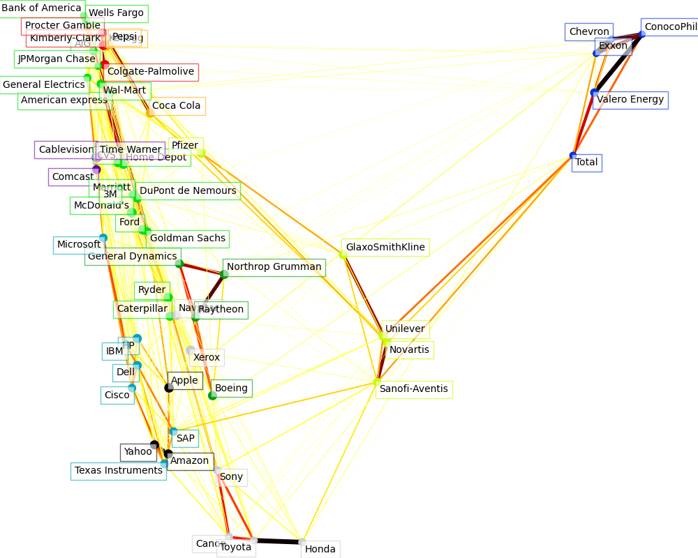
可视化#

3个模型的输出合并到2D图中，其中节点代表股票并边缘连接（偏相关性）：

集群标签用于定义节点的颜色
稀疏协方差模型用于显示边缘的强度
2D嵌入用于定位计划中的节点

此示例包含大量与可视化相关的代码，因为可视化对于显示图形至关重要。挑战之一是放置标签，最大限度地减少重叠。为此，我们使用基于每个轴上最近邻居的方向的启发式方法。

import matplotlib.pyplot as plt
from matplotlib.collections import LineCollection

plt.figure(1, facecolor="w", figsize=(10, 8))
plt.clf()
ax = plt.axes([0.0, 0.0, 1.0, 1.0])
plt.axis("off")

# Plot the graph of partial correlations
partial_correlations = edge_model.precision_.copy()
d = 1 / np.sqrt(np.diag(partial_correlations))
partial_correlations *= d
partial_correlations *= d[:, np.newaxis]
non_zero = np.abs(np.triu(partial_correlations, k=1)) > 0.02

# Plot the nodes using the coordinates of our embedding
plt.scatter(
    embedding[0], embedding[1], s=100 * d**2, c=labels, cmap=plt.cm.nipy_spectral
)

# Plot the edges
start_idx, end_idx = non_zero.nonzero()
# a sequence of (*line0*, *line1*, *line2*), where::
#            linen = (x0, y0), (x1, y1), ... (xm, ym)
segments = [
    [embedding[:, start], embedding[:, stop]] for start, stop in zip(start_idx, end_idx)
]
values = np.abs(partial_correlations[non_zero])
lc = LineCollection(
    segments, zorder=0, cmap=plt.cm.hot_r, norm=plt.Normalize(0, 0.7 * values.max())
)
lc.set_array(values)
lc.set_linewidths(15 * values)
ax.add_collection(lc)

# Add a label to each node. The challenge here is that we want to
# position the labels to avoid overlap with other labels
for index, (name, label, (x, y)) in enumerate(zip(names, labels, embedding.T)):
    dx = x - embedding[0]
    dx[index] = 1
    dy = y - embedding[1]
    dy[index] = 1
    this_dx = dx[np.argmin(np.abs(dy))]
    this_dy = dy[np.argmin(np.abs(dx))]
    if this_dx > 0:
        horizontalalignment = "left"
        x = x + 0.002
    else:
        horizontalalignment = "right"
        x = x - 0.002
    if this_dy > 0:
        verticalalignment = "bottom"
        y = y + 0.002
    else:
        verticalalignment = "top"
        y = y - 0.002
    plt.text(
        x,
        y,
        name,
        size=10,
        horizontalalignment=horizontalalignment,
        verticalalignment=verticalalignment,
        bbox=dict(
            facecolor="w",
            edgecolor=plt.cm.nipy_spectral(label / float(n_labels)),
            alpha=0.6,
        ),
    )

plt.xlim(
    embedding[0].min() - 0.15 * np.ptp(embedding[0]),
    embedding[0].max() + 0.10 * np.ptp(embedding[0]),
)
plt.ylim(
    embedding[1].min() - 0.03 * np.ptp(embedding[1]),
    embedding[1].max() + 0.03 * np.ptp(embedding[1]),
)

plt.show()

Total running time of the script: （0分30.631秒）