梯度提升中的分类特征支持#

在本例中，我们将比较 HistGradientBoostingRegressor 类别特征具有不同的编码策略。特别是，我们将评估：

放弃分类特征
使用 OneHotEncoder
使用 OrdinalEncoder 并将类别视为有序的等距量
使用 OrdinalEncoder 和依靠 native category support 的 HistGradientBoostingRegressor 估计者。

我们将使用艾姆斯爱荷华州住房数据集，该数据集由数字和分类特征组成，其中房屋的销售价格是目标。

看到梯度增强树的梯度中的功能例如，展示的一些其他功能 HistGradientBoostingRegressor .

# Authors: The scikit-learn developers
# SPDX-License-Identifier: BSD-3-Clause

加载Ames Housing数据集#

首先，我们将Ames Housing数据作为pandas框架加载。这些特征要么是分类的，要么是数字的：

from sklearn.datasets import fetch_openml

X, y = fetch_openml(data_id=42165, as_frame=True, return_X_y=True)

# Select only a subset of features of X to make the example faster to run
categorical_columns_subset = [
    "BldgType",
    "GarageFinish",
    "LotConfig",
    "Functional",
    "MasVnrType",
    "HouseStyle",
    "FireplaceQu",
    "ExterCond",
    "ExterQual",
    "PoolQC",
]

numerical_columns_subset = [
    "3SsnPorch",
    "Fireplaces",
    "BsmtHalfBath",
    "HalfBath",
    "GarageCars",
    "TotRmsAbvGrd",
    "BsmtFinSF1",
    "BsmtFinSF2",
    "GrLivArea",
    "ScreenPorch",
]

X = X[categorical_columns_subset + numerical_columns_subset]
X[categorical_columns_subset] = X[categorical_columns_subset].astype("category")

categorical_columns = X.select_dtypes(include="category").columns
n_categorical_features = len(categorical_columns)
n_numerical_features = X.select_dtypes(include="number").shape[1]

print(f"Number of samples: {X.shape[0]}")
print(f"Number of features: {X.shape[1]}")
print(f"Number of categorical features: {n_categorical_features}")
print(f"Number of numerical features: {n_numerical_features}")

Number of samples: 1460
Number of features: 20
Number of categorical features: 10
Number of numerical features: 10

具有删除类别特征的梯度提升估计器#

作为基线，我们创建一个估计器，其中删除分类特征：

from sklearn.compose import make_column_selector, make_column_transformer
from sklearn.ensemble import HistGradientBoostingRegressor
from sklearn.pipeline import make_pipeline

dropper = make_column_transformer(
    ("drop", make_column_selector(dtype_include="category")), remainder="passthrough"
)
hist_dropped = make_pipeline(dropper, HistGradientBoostingRegressor(random_state=42))

具有单热编码的梯度提升估计器#

接下来，我们创建一个管道，该管道将对分类特征进行一次性编码，并让其余的数字数据通过：

from sklearn.preprocessing import OneHotEncoder

one_hot_encoder = make_column_transformer(
    (
        OneHotEncoder(sparse_output=False, handle_unknown="ignore"),
        make_column_selector(dtype_include="category"),
    ),
    remainder="passthrough",
)

hist_one_hot = make_pipeline(
    one_hot_encoder, HistGradientBoostingRegressor(random_state=42)
)

有序编码的梯度提升估计器#

接下来，我们创建一个管道，将分类要素视为有序数量，即类别将被编码为0、1、2等，并被视为连续特征。

import numpy as np

from sklearn.preprocessing import OrdinalEncoder

ordinal_encoder = make_column_transformer(
    (
        OrdinalEncoder(handle_unknown="use_encoded_value", unknown_value=np.nan),
        make_column_selector(dtype_include="category"),
    ),
    remainder="passthrough",
    # Use short feature names to make it easier to specify the categorical
    # variables in the HistGradientBoostingRegressor in the next step
    # of the pipeline.
    verbose_feature_names_out=False,
)

hist_ordinal = make_pipeline(
    ordinal_encoder, HistGradientBoostingRegressor(random_state=42)
)

具有原生类别支持的梯度提升估计器#

我们现在创建一个 HistGradientBoostingRegressor 将本地处理类别特征的估计器。此估计器不会将分类特征视为有序量。我们设定 categorical_features="from_dtype" 使得具有类别d类型的特征被认为是类别特征。

这个估计器与前一个估计器之间的主要区别在于，在这个估计器中，我们让 HistGradientBoostingRegressor 从DataFrame列的dtypes中检测哪些功能是分类的。

hist_native = HistGradientBoostingRegressor(
    random_state=42, categorical_features="from_dtype"
)

模型比较#

最后，我们使用交叉验证来评估模型。在这里，我们从以下方面比较了模型的性能 mean_absolute_percentage_error 和健身时间。

import matplotlib.pyplot as plt

from sklearn.model_selection import cross_validate

scoring = "neg_mean_absolute_percentage_error"
n_cv_folds = 3

dropped_result = cross_validate(hist_dropped, X, y, cv=n_cv_folds, scoring=scoring)
one_hot_result = cross_validate(hist_one_hot, X, y, cv=n_cv_folds, scoring=scoring)
ordinal_result = cross_validate(hist_ordinal, X, y, cv=n_cv_folds, scoring=scoring)
native_result = cross_validate(hist_native, X, y, cv=n_cv_folds, scoring=scoring)


def plot_results(figure_title):
    fig, (ax1, ax2) = plt.subplots(1, 2, figsize=(12, 8))

    plot_info = [
        ("fit_time", "Fit times (s)", ax1, None),
        ("test_score", "Mean Absolute Percentage Error", ax2, None),
    ]

    x, width = np.arange(4), 0.9
    for key, title, ax, y_limit in plot_info:
        items = [
            dropped_result[key],
            one_hot_result[key],
            ordinal_result[key],
            native_result[key],
        ]

        mape_cv_mean = [np.mean(np.abs(item)) for item in items]
        mape_cv_std = [np.std(item) for item in items]

        ax.bar(
            x=x,
            height=mape_cv_mean,
            width=width,
            yerr=mape_cv_std,
            color=["C0", "C1", "C2", "C3"],
        )
        ax.set(
            xlabel="Model",
            title=title,
            xticks=x,
            xticklabels=["Dropped", "One Hot", "Ordinal", "Native"],
            ylim=y_limit,
        )
    fig.suptitle(figure_title)


plot_results("Gradient Boosting on Ames Housing")

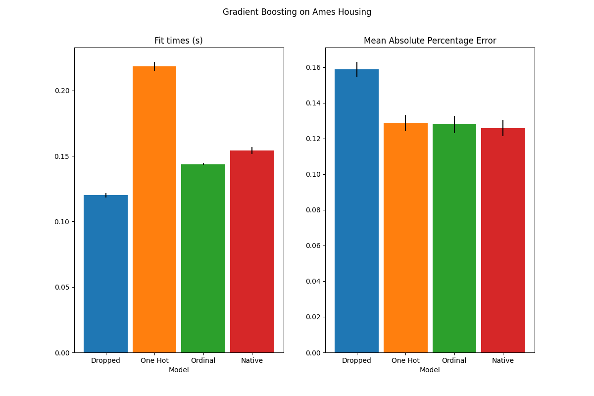
Gradient Boosting on Ames Housing, Fit times (s), Mean Absolute Percentage Error

我们看到，具有单热编码数据的模型是迄今为止最慢的。这是意料之中的，因为一热编码会为每个类别值（对于每个类别特征）创建一个额外的特征，因此在匹配期间需要考虑更多的分裂点。理论上，我们预计类别特征的原生处理会比将类别视为有序量（“有序”）稍微慢一些，因为原生处理需要 sorting categories .然而，当类别数量较少时，调试时间应该很近，但这可能并不总是反映在实践中。

就预测性能而言，放弃分类特征会导致性能较差。使用分类特征的三种模型具有相当的错误率，但原生处理略有优势。

限制拆分次数#

一般来说，人们可以预期单热编码数据的预测较差，尤其是当树深度或节点数量受到限制时：对于单热编码数据，人们需要更多的分裂点，即更多的深度，以便恢复可以在一个单一分裂点中获得的等效分裂。本地处理。

当类别被视为有序量时，这也是如此：如果类别是 A..F 最好的分割是 ACF - BDE 单热编码器模型将需要3个分裂点（左节点中的每个类别一个），而有序非原生模型将需要4个分裂：1个分裂来隔离 A 、1分裂以隔离 F ，并进行2次分裂以隔离 C 从 BCDE .

模型的性能在实践中的差异有多大将取决于数据集和树的灵活性。

为了了解这一点，让我们用欠匹配的模型重新运行相同的分析，其中我们通过限制树的数量和每棵树的深度来人为地限制分裂的总数。

for pipe in (hist_dropped, hist_one_hot, hist_ordinal, hist_native):
    if pipe is hist_native:
        # The native model does not use a pipeline so, we can set the parameters
        # directly.
        pipe.set_params(max_depth=3, max_iter=15)
    else:
        pipe.set_params(
            histgradientboostingregressor__max_depth=3,
            histgradientboostingregressor__max_iter=15,
        )

dropped_result = cross_validate(hist_dropped, X, y, cv=n_cv_folds, scoring=scoring)
one_hot_result = cross_validate(hist_one_hot, X, y, cv=n_cv_folds, scoring=scoring)
ordinal_result = cross_validate(hist_ordinal, X, y, cv=n_cv_folds, scoring=scoring)
native_result = cross_validate(hist_native, X, y, cv=n_cv_folds, scoring=scoring)

plot_results("Gradient Boosting on Ames Housing (few and small trees)")

plt.show()

Gradient Boosting on Ames Housing (few and small trees), Fit times (s), Mean Absolute Percentage Error

这些欠拟模型的结果证实了我们之前的直觉：当拆分预算受到限制时，原生类别处理策略表现最好。另外两种策略（一热编码和将类别视为有序值）导致的误差值与刚刚完全放弃类别特征的基线模型相当。

Total running time of the script: （0分2.564秒）