1.11. 合奏:梯度提升、随机森林、装袋、投票、堆叠#
Ensemble methods 结合使用给定学习算法构建的几个基本估计器的预测,以提高单个估计器的可推广性/鲁棒性。
集成方法的两个非常著名的例子是 gradient-boosted trees 和 random forests .
更一般地说,集成模型可以应用于树以外的任何基本学习器,采用平均方法,例如 Bagging methods , model stacking ,或者 Voting ,或在升压中,如 AdaBoost .
1.11.1. 受影响的树木#
Gradient Tree Boosting 或梯度增强决策树(GBDT)是增强到任意可微损失函数的概括,请参阅 [Friedman2001]. GBDT是回归和分类的优秀模型,尤其是对于表格数据。
1.11.1.1. 基于直方图的梯度提升#
Scikit-learn 0.21引入了两种新的梯度增强树实现,即 HistGradientBoostingClassifier 和 HistGradientBoostingRegressor ,灵感来自 LightGBM (见 [LightGBM]) .
这些基于柱状图的估计值可以是 orders of magnitude faster 比 GradientBoostingClassifier 和 GradientBoostingRegressor 当样本数量大于数万个样本时。
它们还内置了对缺失值的支持,从而避免了对估算器的需要。
这些快速估计器首先对输入样本进行分类 X 转换为整值箱(通常为256个箱),这极大地减少了需要考虑的分裂点的数量,并允许算法在构建树时利用基于整值的数据结构(柱状图),而不是依赖于排序的连续值。这些估计器的API略有不同,并且来自 GradientBoostingClassifier 和 GradientBoostingRegressor 尚未支持,例如一些丢失功能。
示例
sphx_glr_auto_examples_inspection_plot_partial_dependence.py
1.11.1.1.1. 使用#
大部分参数与 GradientBoostingClassifier 和 GradientBoostingRegressor .一个例外是 max_iter 替换的参数 n_estimators ,并控制助推过程的迭代次数::
>>> from sklearn.ensemble import HistGradientBoostingClassifier
>>> from sklearn.datasets import make_hastie_10_2

>>> X, y = make_hastie_10_2(random_state=0)
>>> X_train, X_test = X[:2000], X[2000:]
>>> y_train, y_test = y[:2000], y[2000:]

>>> clf = HistGradientBoostingClassifier(max_iter=100).fit(X_train, y_train)
>>> clf.score(X_test, y_test)
0.8965
可用损失 regression 是:
“squared_error”,这是默认损失;
“absolute_error”,它对异常值的敏感性低于平方误差;
“伽玛”,非常适合对严格的积极结果进行建模;
“泊松”,非常适合模型计数和频率;
“分位数”,它允许估计条件分位数,稍后可用于获得预测区间。
为 classification ,“log_loss”是唯一的选项。对于二进制分类,它使用二进制log损失,也称为二项偏差或二进制交叉熵。为 n_classes >= 3 ,它使用多类日志损失函数,并以多项偏差和类别交叉信息作为替代名称。根据以下因素选择合适的丢失版本 y 传递给 fit .
树木的大小可以通过 max_leaf_nodes , max_depth ,而且 min_samples_leaf 参数
用于对数据进行分类的分类器数量由 max_bins 参数.使用更少的箱可以作为一种正规化形式。通常建议使用尽可能多的垃圾箱(255),这是默认情况。
的 l2_regularization 参数充当损失函数的正规化器,对应于 \(\lambda\) 在下面的公式中(参见中的公式(2) [XGBoost]) :
L2正则化的细节#
重要的是要注意, \(l(\hat{y}_i, y_i)\) 只描述了实际损失函数的一半,除了弹球损失和绝对误差。
该指数 \(k\) 指的是树集合中的第k棵树。在回归和二元分类的情况下,梯度提升模型每次迭代生长一棵树,然后 \(k\) 跑到 max_iter .在多类分类问题的情况下,指数的最大值 \(k\) 是 n_classes \(\times\) max_iter .
如果 \(T_k\) 表示第k棵树中的叶子数量,那么 \(w_k\) 是长度的载体 \(T_k\) ,其中包含形式的叶值 w = -sum_gradient / (sum_hessian + l2_regularization) (see方程(5), [XGBoost]) .
The leaf values \(w_k\) are derived by dividing the sum of the gradients of the loss function by the combined sum of hessians. Adding the regularization to the denominator penalizes the leaves with small hessians (flat regions), resulting in smaller updates. Those \(w_k\) values contribute then to the model's prediction for a given input that ends up in the corresponding leaf. The final prediction is the sum of the base prediction and the contributions from each tree. The result of that sum is then transformed by the inverse link function depending on the choice of the loss function (see 数学公式).
请注意原始论文 [XGBoost] 引入一个术语 \(\gamma\sum_k T_k\) 这会惩罚叶子的数量(使其成为平滑版本 max_leaf_nodes )此处未呈现,因为它未在scikit-learn中实现;而 \(\lambda\) 在根据学习率重新缩放之前惩罚单个树预测的幅度,请参阅 Shrinkage via learning rate .
注意 early-stopping is enabled by default if the number of samples is larger than 10,000 .提前停止行为通过控制 early_stopping , scoring , validation_fraction , n_iter_no_change ,而且 tol 参数可以提前停止使用任意的 scorer ,或者只是培训或验证损失。请注意,由于技术原因,使用可调用作为得分器明显比使用损失慢。默认情况下,如果训练集中至少有10,000个样本,则使用验证损失执行提前停止。
1.11.1.1.2. 缺失值支持#
HistGradientBoostingClassifier 和 HistGradientBoostingRegressor 内置对缺失值(NaN)的支持。
在训练过程中,树木种植者根据潜在的收益,在每个分裂点学习缺失值的样本是否应该流向左孩子还是右孩子。预测时,具有缺失值的样本将被分配给左或右子项:
>>> from sklearn.ensemble import HistGradientBoostingClassifier
>>> import numpy as np

>>> X = np.array([0, 1, 2, np.nan]).reshape(-1, 1)
>>> y = [0, 0, 1, 1]

>>> gbdt = HistGradientBoostingClassifier(min_samples_leaf=1).fit(X, y)
>>> gbdt.predict(X)
array([0, 0, 1, 1])
当缺失模式是预测性的时,可以对特征值是否缺失执行拆分::
>>> X = np.array([0, np.nan, 1, 2, np.nan]).reshape(-1, 1)
>>> y = [0, 1, 0, 0, 1]
>>> gbdt = HistGradientBoostingClassifier(min_samples_leaf=1,
...                                       max_depth=2,
...                                       learning_rate=1,
...                                       max_iter=1).fit(X, y)
>>> gbdt.predict(X)
array([0, 1, 0, 0, 1])
如果在训练期间没有遇到给定特征的缺失值,则具有缺失值的样本将映射到具有最多样本的孩子。
示例
1.11.1.1.3. 样本重量支持#
HistGradientBoostingClassifier 和 HistGradientBoostingRegressor 支持样品重量, fit .
下面的玩具示例演示了样本权重为零的样本将被忽略:
>>> X = [[1, 0],
...      [1, 0],
...      [1, 0],
...      [0, 1]]
>>> y = [0, 0, 1, 0]
>>> # ignore the first 2 training samples by setting their weight to 0
>>> sample_weight = [0, 0, 1, 1]
>>> gb = HistGradientBoostingClassifier(min_samples_leaf=1)
>>> gb.fit(X, y, sample_weight=sample_weight)
HistGradientBoostingClassifier(...)
>>> gb.predict([[1, 0]])
array([1])
>>> gb.predict_proba([[1, 0]])[0, 1]
np.float64(0.999)
如你所见 [1, 0] 被轻松归类为 1 因为前两个样本由于其样本权重而被忽略。
实现细节:考虑样本权重相当于将梯度(和粗线)乘以样本权重。请注意,分类阶段(特别是分位数计算)不考虑权重。
1.11.1.1.4. 类别功能支持#
HistGradientBoostingClassifier 和 HistGradientBoostingRegressor 对分类功能具有原生支持:他们可以考虑对无序的分类数据进行拆分。
对于具有分类特征的数据集,使用原生分类支持通常比依赖单一编码更好 (OneHotEncoder ),因为单热编码需要更多的树深度才能实现等效的拆分。通常最好依赖原生类别支持,而不是将类别特征视为连续(有序),这种情况适用于有序编码的类别数据,因为类别是名义量,其中顺序并不重要。
要启用分类支持,可以将布尔屏蔽传递给 categorical_features 参数,指示哪个特征是分类的。在下文中,第一个特征将被视为类别特征,第二个特征将被视为数字特征::
>>> gbdt = HistGradientBoostingClassifier(categorical_features=[True, False])
等效地,可以传递指示分类特征索引的一系列整元::
>>> gbdt = HistGradientBoostingClassifier(categorical_features=[0])
当输入是DataFrame时,也可以传递一个列名列表::
>>> gbdt = HistGradientBoostingClassifier(categorical_features=["site", "manufacturer"])
最后,当输入是DataFrame时,我们可以使用 categorical_features="from_dtype" 在这种情况下,所有包含类别的列 dtype 将被视为分类特征。
每个类别特征的基数必须小于 max_bins 参数.有关对分类要素使用基于柱状图的梯度增强的示例,请参阅 梯度提升中的分类特征支持 .
如果训练期间存在缺失值,则缺失值将被视为适当的类别。如果训练期间没有缺失值,那么在预测时,缺失值将被映射到具有最多样本的子节点(就像连续特征一样)。预测时,在适应时间内未看到的类别将被视为缺失值。
具有类别特征的分裂发现#
The canonical way of considering categorical splits in a tree is to consider
all of the \(2^{K - 1} - 1\) partitions, where \(K\) is the number of
categories. This can quickly become prohibitive when \(K\) is large.
Fortunately, since gradient boosting trees are always regression trees (even
for classification problems), there exists a faster strategy that can yield
equivalent splits. First, the categories of a feature are sorted according to
the variance of the target, for each category k. Once the categories are
sorted, one can consider continuous partitions, i.e. treat the categories
as if they were ordered continuous values (see Fisher [Fisher1958] for a
formal proof). As a result, only \(K - 1\) splits need to be considered
instead of \(2^{K - 1} - 1\). The initial sorting is a
\(\mathcal{O}(K \log(K))\) operation, leading to a total complexity of
\(\mathcal{O}(K \log(K) + K)\), instead of \(\mathcal{O}(2^K)\).
示例
1.11.1.1.5. 单调约束#
根据当前的问题,您可能有先验知识表明给定功能通常应该对目标值产生积极(或消极)影响。例如,在其他条件相同的情况下,较高的信用评分应该会增加获得贷款批准的可能性。单调约束允许您将此类先验知识融入到模型中。
对于预测者 \(F\) 有两个特点:
一 monotonic increase constraint 是形式的约束:
\[x_1 \leq x_1 '\暗示F(x_1,x_2)\leq F(x_1 ',x_2)\]一 monotonic decrease constraint 是形式的约束:
\[x_1 \leq x_1 '\暗示F(x_1,x_2)\geq F(x_1 ',x_2)\]
属性为每个要素指定单调约束 monotonic_cst 参数.对于每个特征,值0表示没有约束,而1和-1分别表示单调增加和单调减少约束::
>>> from sklearn.ensemble import HistGradientBoostingRegressor

... # monotonic increase, monotonic decrease, and no constraint on the 3 features
>>> gbdt = HistGradientBoostingRegressor(monotonic_cst=[1, -1, 0])
在二元分类上下文中,施加单调增加(减少)约束意味着更高的特征值应该对样本属于正类的概率产生正(负)影响。
然而,单调约束只能在一定程度上限制特征对输出的影响。例如,单调增加和减少约束不能用于强制执行以下建模约束:
此外,多类分类不支持单调约束。
备注
由于类别是无序量,因此不可能对类别特征强制单调约束。
示例
1.11.1.1.6. 互动限制#
先验地,允许使用任何特征将节点拆分为子节点。这会在功能之间创建所谓的交互,即沿着分支分裂的不同功能的使用。有时,人们想要限制可能的互动,请参阅 [Mayer2022]. 这可以通过参数来完成 interaction_cst ,其中可以指定允许交互的特征的索引。例如,总共有3个功能, interaction_cst=[{0}, {1}, {2}] 禁止所有互动。的约束 [{0, 1}, {1, 2}] 指定两组可能相互作用的功能。特征0和1可以相互作用,特征1和2也可以相互作用。但请注意,功能0和2禁止交互。以下描述了一棵树和树可能的分裂:
   1      <- Both constraint groups could be applied from now on
  / \
 1   2    <- Left split still fulfills both constraint groups.
/ \ / \      Right split at feature 2 has only group {1, 2} from now on.
LightGBM对重叠组使用相同的逻辑。
请注意,未列出的功能 interaction_cst 会自动为自己分配一个互动组。再次有3个功能,这意味着 [{0}] 相当于 [{0}, {1, 2}] .
示例
sphx_glr_auto_examples_inspection_plot_partial_dependence.py
引用
M.梅耶尔,南卡罗来纳州布拉萨,M.霍伊斯利和DF斯科纳米利奥。2022. Machine Learning Applications to Land and Structure Valuation .风险与财务管理杂志15,第5期:193
1.11.1.1.7. 低级并行#
HistGradientBoostingClassifier 和 HistGradientBoostingRegressor 使用MEK通过Cython进行并行化。有关如何控制线程数的更多详细信息,请参阅我们的 并行性 notes.
以下部分是并行的:
将样本从实值映射到整值箱(但找到箱阈值是连续的)
建筑矩形图在要素上并行化
在节点上查找最佳分割点是在要素上并行进行的
在匹配过程中,将样本映射到左子和右子部分是在样本上并行的
梯度和黑森计算在样本上并行化
预测在样本上并行进行
1.11.1.1.8. 为什么它更快#
The bottleneck of a gradient boosting procedure is building the decision
trees. Building a traditional decision tree (as in the other GBDTs
GradientBoostingClassifier and GradientBoostingRegressor)
requires sorting the samples at each node (for
each feature). Sorting is needed so that the potential gain of a split point
can be computed efficiently. Splitting a single node has thus a complexity
of \(\mathcal{O}(n_\text{features} \times n \log(n))\) where \(n\)
is the number of samples at the node.
HistGradientBoostingClassifier and
HistGradientBoostingRegressor, in contrast, do not require sorting the
feature values and instead use a data-structure called a histogram, where the
samples are implicitly ordered. Building a histogram has a
\(\mathcal{O}(n)\) complexity, so the node splitting procedure has a
\(\mathcal{O}(n_\text{features} \times n)\) complexity, much smaller
than the previous one. In addition, instead of considering \(n\) split
points, we consider only max_bins split points, which might be much
smaller.
为了构建图表,输入数据 X 需要被分类到整值箱中。此分类过程确实需要对要素值进行排序,但它只在提升过程的一开始发生一次(不是在每个节点上,就像在 GradientBoostingClassifier 和 GradientBoostingRegressor ).
Finally, many parts of the implementation of
HistGradientBoostingClassifier and
HistGradientBoostingRegressor are parallelized.
引用
Fisher,W.D.(1958)。 "On Grouping for Maximum Homogeneity" 美国统计协会杂志,53,789-798。
1.11.1.2. GradientBoostingClassifier 和 GradientBoostingRegressor#
的用途和参数 GradientBoostingClassifier 和 GradientBoostingRegressor 如下所述。这些估计量的2个最重要的参数是 n_estimators 和 learning_rate .
分类#
GradientBoostingClassifier 支持二进制和多类分类。下面的示例展示了如何将具有100个决策树桩的梯度增强分类器匹配为弱学习者::
>>> from sklearn.datasets import make_hastie_10_2
>>> from sklearn.ensemble import GradientBoostingClassifier

>>> X, y = make_hastie_10_2(random_state=0)
>>> X_train, X_test = X[:2000], X[2000:]
>>> y_train, y_test = y[:2000], y[2000:]

>>> clf = GradientBoostingClassifier(n_estimators=100, learning_rate=1.0,
...     max_depth=1, random_state=0).fit(X_train, y_train)
>>> clf.score(X_test, y_test)
0.913
弱学习器(即回归树)的数量由参数控制 n_estimators ; The size of each tree 可以通过设置树木深度来控制 max_depth 或通过设置叶节点的数量 max_leaf_nodes .的 learning_rate 是范围(0.0,1.0)内的超参数,通过以下方式控制过逼近 shrinkage .
备注
超过2个类别的分类需要归纳 n_classes 每次迭代时的回归树,因此,诱导树的总数等于 n_classes * n_estimators .对于具有大量类的数据集,我们强烈建议使用 HistGradientBoostingClassifier 作为替代 GradientBoostingClassifier .
回归#
GradientBoostingRegressor supports a number of
different loss functions
for regression which can be specified via the argument
loss; the default loss function for regression is squared error
('squared_error').
>>> import numpy as np
>>> from sklearn.metrics import mean_squared_error
>>> from sklearn.datasets import make_friedman1
>>> from sklearn.ensemble import GradientBoostingRegressor

>>> X, y = make_friedman1(n_samples=1200, random_state=0, noise=1.0)
>>> X_train, X_test = X[:200], X[200:]
>>> y_train, y_test = y[:200], y[200:]
>>> est = GradientBoostingRegressor(
...     n_estimators=100, learning_rate=0.1, max_depth=1, random_state=0,
...     loss='squared_error'
... ).fit(X_train, y_train)
>>> mean_squared_error(y_test, est.predict(X_test))
5.00
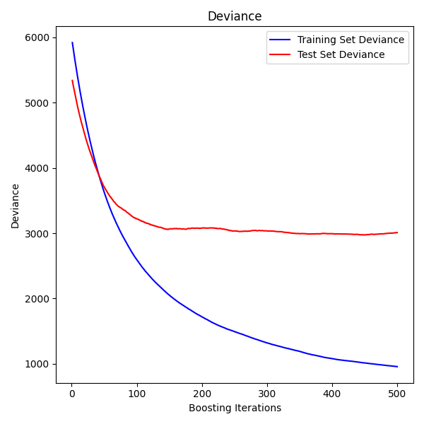
下图显示了应用结果 GradientBoostingRegressor 糖尿病数据集的最小平方损失和500个基本学习者 (sklearn.datasets.load_diabetes ).该图显示了每次迭代时的训练和测试误差。每次迭代时的训练误差都存储在 train_score_ 梯度提升模型的属性。每次迭代的测试误差可以通过 staged_predict 方法,该方法返回生成器,该生成器在每个阶段产生预测。像这样的地块可用于确定树的最佳数量(即 n_estimators )通过提前停止。
示例
1.11.1.2.1. 培养更多的学习能力较差的人#
两 GradientBoostingRegressor 和 GradientBoostingClassifier 支持 warm_start=True 这允许您向已经匹配的模型添加更多估计量。
>>> import numpy as np
>>> from sklearn.metrics import mean_squared_error
>>> from sklearn.datasets import make_friedman1
>>> from sklearn.ensemble import GradientBoostingRegressor

>>> X, y = make_friedman1(n_samples=1200, random_state=0, noise=1.0)
>>> X_train, X_test = X[:200], X[200:]
>>> y_train, y_test = y[:200], y[200:]
>>> est = GradientBoostingRegressor(
...     n_estimators=100, learning_rate=0.1, max_depth=1, random_state=0,
...     loss='squared_error'
... )
>>> est = est.fit(X_train, y_train)  # fit with 100 trees
>>> mean_squared_error(y_test, est.predict(X_test))
5.00
>>> _ = est.set_params(n_estimators=200, warm_start=True)  # set warm_start and increase num of trees
>>> _ = est.fit(X_train, y_train) # fit additional 100 trees to est
>>> mean_squared_error(y_test, est.predict(X_test))
3.84
1.11.1.2.2. 控制树木大小#
回归树基学习器的大小定义了梯度提升模型可以捕获的变量交互的水平。一般来说,深度之树 h 可以捕捉秩序的互动 h .有两种方法可以控制单个回归树的大小。
如果指定 max_depth=h 然后完成深度的二元树 h 将会成长。这样的树(最多) 2**h 叶节点和 2**h - 1 分割节点。
或者,您可以通过参数指定叶节点的数量来控制树大小 max_leaf_nodes .在这种情况下,将使用最佳优先搜索来生长树木,其中杂质改进最高的节点将首先被扩展。一棵树 max_leaf_nodes=k 具有 k - 1 拆分节点,因此可以对高级别的交互进行建模 max_leaf_nodes - 1 .
我们发现 max_leaf_nodes=k 给出了与之相当的结果 max_depth=k-1 但训练速度明显更快,但训练误差稍高。参数 max_leaf_nodes 对应于变量 J 在关于梯度增强的章节中 [Friedman2001] 并且与参数相关 interaction.depth 在R的gbm包中, max_leaf_nodes == interaction.depth + 1 .
1.11.1.2.3. 数学公式#
我们首先介绍GBRT进行回归,然后详细介绍分类案例。
回归#
GBRT regressors are additive models whose prediction \(\hat{y}_i\) for a given input \(x_i\) is of the following form:
其中 \(h_m\) 被称为估计器 weak learners 在助推的背景下。渐变树增强用途 decision tree regressors 作为弱学习者,其规模固定。常数M对应于 n_estimators 参数.
与其他提升算法类似,GBRT是以贪婪的方式构建的:
新增加的树 \(h_m\) 安装是为了最大限度地减少损失 \(L_m\) 考虑到之前的合奏, \(F_{m-1}\) :
哪里 \(l(y_i, F(x_i))\) 所限定 loss 参数,在下一节详细介绍。
默认情况下,初始模型 \(F_{0}\) 选择作为最小化损失的常数:对于最小平方损失,这是目标值的经验平均值。初始模型也可以通过指定 init 论点
使用一阶泰勒逼近, \(l\) 可以大致如下:
备注
Briefly, a first-order Taylor approximation says that \(l(z) \approx l(a) + (z - a) \frac{\partial l}{\partial z}(a)\). Here, \(z\) corresponds to \(F_{m - 1}(x_i) + h_m(x_i)\), and \(a\) corresponds to \(F_{m-1}(x_i)\)
The quantity \(\left[ \frac{\partial l(y_i, F(x_i))}{\partial F(x_i)} \right]_{F=F_{m - 1}}\) is the derivative of the loss with respect to its second parameter, evaluated at \(F_{m-1}(x)\). It is easy to compute for any given \(F_{m - 1}(x_i)\) in a closed form since the loss is differentiable. We will denote it by \(g_i\).
除去常项,我们有:
This is minimized if \(h(x_i)\) is fitted to predict a value that is proportional to the negative gradient \(-g_i\). Therefore, at each iteration, the estimator \(h_m\) is fitted to predict the negative gradients of the samples. The gradients are updated at each iteration. This can be considered as some kind of gradient descent in a functional space.
备注
对于一些损失,例如 'absolute_error' 梯度在哪里 \(\pm 1\) ,由一个匹配的预测值 \(h_m\) 不够准确:树只能输出integer值。结果,树的叶子值 \(h_m\) 一旦树被匹配,就会进行修改,以便叶子值将损失最小化 \(L_m\) .更新取决于损失:对于绝对误差损失,叶的值被更新为该叶中样本的中位数。
分类#
分类的梯度增强与回归情况非常相似。然而,树木的总和 \(F_M(x_i) = \sum_m h_m(x_i)\) 与预测不同质:它不能是一个类,因为树预测连续值。
从值的映射 \(F_M(x_i)\) 对于一类或概率是依赖于损失的。对于log损失,是指 \(x_i\) 属于正类的建模为 \(p(y_i = 1 | x_i) = \sigma(F_M(x_i))\) 哪里 \(\sigma\) 是Sigmoid或expit函数。
对于多类分类,在每个 \(M\) 迭代。的概率 \(x_i\) 属于类k被建模为 \(F_{M,k}(x_i)\) 价值观
请注意,即使对于分类任务, \(h_m\) 子估计器仍然是回归量,而不是分类器。这是因为子估计器经过训练以预测(负) gradients ,它们始终是连续的量。
1.11.1.2.4. 损失函数#
支持以下损失函数,并且可以使用参数指定 loss :
回归#
方误差 (
'squared_error'):由于其优越的计算特性,回归的自然选择。初始模型由目标值的平均值给出。绝对误差 (
'absolute_error'):稳健的回归损失函数。初始模型由目标值的中位数给出。Huber (
'huber'):另一个结合了最小平方和最小绝对偏差的稳健损失函数;使用alpha控制异常值的敏感性(请参阅 [Friedman2001] 了解更多详情)。分位 (
'quantile'):分位数回归的损失函数。使用0 < alpha < 1以指定分位数。此损失函数可用于创建预测区间(请参阅 梯度Boosting回归的预测区间 ).
分类#
二进制log损失 (
'log-loss'):二进制分类的二项负log似然损失函数。它提供了可能性估计。 初始模型由log赔率比给出。多类日志损失 (
'log-loss'):用于多类分类的多项负对log似然损失函数,n_classes相互排斥的类。它提供了可能性估计。 初始模型由每个类别的先验概率给出。在每次迭代时n_classes必须构建回归树,这使得GBRT对于具有大量类的数据集来说效率相当低。指数损失 (
'exponential'):与相同的损失函数AdaBoostClassifier.对于错误标签的示例来说,'log-loss';仅可用于二进制分类。
1.11.1.2.5. Shrinkage via learning rate#
[Friedman2001] 提出了一种简单的正规化策略,通过一个恒定因子来缩放每个弱学习者的贡献 \(\nu\) :
参数 \(\nu\) 也被称为 learning rate 因为它扩展了梯度下降过程的步进长度;它可以通过 learning_rate 参数.
参数 learning_rate 与参数强烈相互作用 n_estimators ,需要适应的弱学习者数量。的较小值 learning_rate 需要大量的弱学习者来保持持续的训练误差。经验证据表明, learning_rate 支持更好的测试错误。 [HTF] 建议将学习率设置为一个小常数(例如, learning_rate <= 0.1 )并选择 n_estimators 足够大,可以提前停止,请参阅 Gradient Boosting中的提前停止 以更详细地讨论 learning_rate 和 n_estimators 看到 [R2007].
1.11.1.2.6. 子采样#
[Friedman2002] 提出了随机梯度提升,将梯度提升与自举平均(bagging)相结合。在每次迭代时,基本分类器都会在分数上训练 subsample 可用的训练数据。子样本是在不替换的情况下绘制的。的典型值 subsample 是0.5。
下图说明了收缩和二次抽样对模型适合度的影响。我们可以清楚地看到,收缩优于无收缩。带收缩的二次抽样可以进一步提高模型的准确性。另一方面,没有收缩的二次抽样效果不佳。
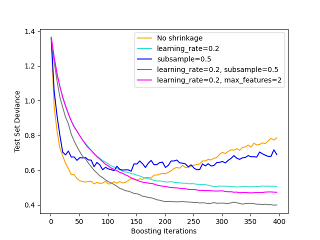
另一种减少方差的策略是通过对特征进行二次采样,类似于 RandomForestClassifier .二次采样要素的数量可以通过 max_features 参数.
备注
使用小 max_features 值可以显着减少运行时间。
随机梯度提升允许通过计算未包含在引导样本中的示例(即袋外示例)的偏差改进来计算测试偏差的袋外估计。改进存储在属性中 oob_improvement_ . oob_improvement_[i] 如果将第i个阶段添加到当前预测中,则可以保持在OSC样本损失方面的改进。袋外估计可用于模型选择,例如确定最佳迭代次数。OOB估计通常非常悲观,因此我们建议使用交叉验证,并且只有在交叉验证太耗时时才使用OOB。
示例
1.11.1.2.7. Interpretation with feature importance#
通过简单地可视化树结构,就可以轻松地解释单个决策树。然而,梯度提升模型由数百棵回归树组成,因此无法通过对单个树的视觉检查来轻松解释它们。幸运的是,人们提出了许多技术来总结和解释梯度增强模型。
通常,特征对预测目标响应的贡献并不相等;在许多情况下,大多数特征实际上是不相关的。在解释一个模型时,第一个问题通常是:这些重要的特征是什么?它们如何有助于预测目标反应?
个体决策树本质上通过选择适当的分裂点来执行特征选择。该信息可用于衡量每个特征的重要性;基本思想是:一个特征在树的分裂点中使用的频率越高,该特征就越重要。通过简单地平均每棵树的基于杂质的特征重要性,这种重要性概念可以扩展到决策树集合(请参阅 特征重要性评价 了解更多详情)。
适合梯度增强模型的特征重要性分数可以通过 feature_importances_ 属性::
>>> from sklearn.datasets import make_hastie_10_2
>>> from sklearn.ensemble import GradientBoostingClassifier

>>> X, y = make_hastie_10_2(random_state=0)
>>> clf = GradientBoostingClassifier(n_estimators=100, learning_rate=1.0,
...     max_depth=1, random_state=0).fit(X, y)
>>> clf.feature_importances_
array([0.107, 0.105, 0.113, 0.0987, 0.0947,
       0.107, 0.0916, 0.0972, 0.0958, 0.0906])
请注意,这种特征重要性的计算是基于信息量的,并且与信息量不同 sklearn.inspection.permutation_importance 这是基于特征的排列。
示例
引用
Friedman,J.H.(2001)。 Greedy function approximation: A gradient boosting machine .《统计年鉴》,29,1189-1232。
Friedman,J.H.(2002)。 Stochastic gradient boosting. .计算统计与数据分析,38,367-378。
G. Ridgeway (2006). Generalized Boosted Models: A guide to the gbm package
1.11.2. 随机森林和其他随机树木群落#
的 sklearn.ensemble 模块包括两个平均算法的基础上随机 decision trees :RandomForest算法和Extra Trees方法。这两种算法都是扰动合并技术 [B1998] 专门为树木设计。这意味着通过在分类器构造中引入随机性来创建多样化的分类器集。 集合的预测作为各个分类器的平均预测给出。
与其他分类器一样,森林分类器必须配备两个数组:形状的稀疏或密集数组X (n_samples, n_features) 保存训练样本和形状的阵列Y (n_samples,) 保存训练样本的目标值(类别标签)::
>>> from sklearn.ensemble import RandomForestClassifier
>>> X = [[0, 0], [1, 1]]
>>> Y = [0, 1]
>>> clf = RandomForestClassifier(n_estimators=10)
>>> clf = clf.fit(X, Y)
像 decision trees 树木森林也延伸到 multi-output problems (if Y是一个形状数组 (n_samples, n_outputs) ).
1.11.2.1. 随机森林#
在随机森林中(请参阅 RandomForestClassifier 和 RandomForestRegressor 类),系综中的每棵树都是从利用替换绘制的样本构建的(即,Bootstrap样本)。
此外,当在树的构建过程中拆分每个节点时,通过对所有输入要素或随机大小子集的特征值进行详尽搜索来找到最佳拆分 max_features . (See的 parameter tuning guidelines 了解更多详细信息。)
这两个随机性来源的目的是减少森林估计器的方差。事实上,单个决策树通常表现出很高的方差并且倾向于过适应。注入森林的随机性会产生具有一定程度上脱钩的预测误差的决策树。通过取这些预测的平均值,一些错误可以抵消。随机森林通过组合不同的树木来减少方差,有时以偏差略有增加为代价。在实践中,方差减少通常是显着的,因此产生了总体更好的模型。
与原始出版物相反 [B2001], scikit-learn实现通过平均概率预测来组合分类器,而不是让每个分类器投票给单个类别。
随机森林的一个有竞争力的替代方案是 基于直方图的梯度提升 (HGBT)型号:
建造树木:随机森林通常依赖于深树(单独过度匹配),这会使用大量计算资源,因为它们需要多次分裂和对候选分裂的评估。增强模型会构建浅树(单独不适合),这些树可以更快地适应和预测。
顺序提升:在HGBT中,决策树是顺序构建的,其中每棵树都经过训练以纠正前几棵树造成的错误。这使得他们能够使用相对较少的树迭代地改进模型的性能。相比之下,随机森林使用多数票来预测结果,这可能需要更多数量的树木才能实现相同水平的准确性。
高效的装箱:HGBT使用高效的装箱算法,可以处理具有大量特征的大型数据集。分箱算法可以预处理数据,以加快后续的树构建(请参见 Why it's faster ).相比之下,随机森林的scikit-learn实现不使用分类,而是依赖于精确的拆分,这在计算上可能很昂贵。
总体而言,HGBT与RF的计算成本取决于数据集和建模任务的具体特征。尝试这两种模型并比较它们在特定问题上的性能和计算效率,以确定哪个模型最适合。
示例
1.11.2.2. 极度随机的树木#
在极其随机的树中(请参阅 ExtraTreesClassifier 和 ExtraTreesRegressor 类),随机性在计算分裂的方式上更进一步。与随机森林一样,使用候选特征的随机子集,但不是寻找最具区分性的阈值,而是为每个候选特征随机绘制阈值,并选择这些随机生成的阈值中的最佳阈值作为分裂规则。这通常允许更多地减少模型的方差,但以偏差稍微增加为代价::
>>> from sklearn.model_selection import cross_val_score
>>> from sklearn.datasets import make_blobs
>>> from sklearn.ensemble import RandomForestClassifier
>>> from sklearn.ensemble import ExtraTreesClassifier
>>> from sklearn.tree import DecisionTreeClassifier

>>> X, y = make_blobs(n_samples=10000, n_features=10, centers=100,
...     random_state=0)

>>> clf = DecisionTreeClassifier(max_depth=None, min_samples_split=2,
...     random_state=0)
>>> scores = cross_val_score(clf, X, y, cv=5)
>>> scores.mean()
np.float64(0.98)

>>> clf = RandomForestClassifier(n_estimators=10, max_depth=None,
...     min_samples_split=2, random_state=0)
>>> scores = cross_val_score(clf, X, y, cv=5)
>>> scores.mean()
np.float64(0.999)

>>> clf = ExtraTreesClassifier(n_estimators=10, max_depth=None,
...     min_samples_split=2, random_state=0)
>>> scores = cross_val_score(clf, X, y, cv=5)
>>> scores.mean() > 0.999
np.True_
1.11.2.3. 参数#
使用这些方法时需要调整的主要参数是 n_estimators 和 max_features .前者是森林中树木的数量。越大越好,但计算所需的时间也越长。此外,请注意,超过临界数量的树木后,结果将停止显着改善。后者是分裂节点时要考虑的随机特征子集的大小。方差的减少越大,但偏差的增加也越大。经验良好的违约值是 max_features=1.0 或等效地 max_features=None (始终考虑所有特征而不是随机子集)用于回归问题,以及 max_features="sqrt" (使用大小的随机子集 sqrt(n_features) )用于分类任务(其中 n_features 是数据中的特征数量)。的默认值 max_features=1.0 相当于袋装树,通过设置较小的值可以实现更多随机性(例如,0.3是文献中典型的默认值)。设置时往往会取得良好的效果 max_depth=None 结合 min_samples_split=2 (i.e.,当树木完全发育时)。但请记住,这些值通常不是最佳值,并且可能会导致模型消耗大量RAM。最佳参数值应始终进行交叉验证。此外,请注意,在随机森林中,默认使用Bootstrap样本 (bootstrap=True )而额外树的默认策略是使用整个数据集 (bootstrap=False ).当使用自举抽样时,可以在遗漏或袋外样本上估计概括误差。这可以通过设置来启用 oob_score=True .
备注
具有默认参数的模型大小为 \(O( M * N * log (N) )\) ,在哪里 \(M\) 是树木的数量和 \(N\) 是样本数量。为了缩小模型的大小,您可以更改这些参数: min_samples_split , max_leaf_nodes , max_depth 和 min_samples_leaf .
1.11.2.4. 并行化#
最后,该模块还具有树的并行构建以及通过 n_jobs 参数.如果 n_jobs=k 然后计算被划分为 k 工作,并继续运行 k 机器的核心。如果 n_jobs=-1 然后使用机器上可用的所有核心。请注意,由于进程间通信负担,加速可能不是线性的(即,使用 k 不幸的是,工作不会 k 时间一样快)。尽管当构建大量树时,或者当构建单个树需要相当长的时间时(例如,在大型数据集上)。
示例
引用
P. Geurts, D. Ernst., and L. Wehenkel, "Extremely randomized trees", Machine Learning, 63(1), 3-42, 2006.
1.11.2.5. 特征重要性评价#
用作树中决策节点的特征的相对排名(即深度)可用于评估该特征相对于目标变量的可预测性的相对重要性。树顶部使用的特征有助于更大部分输入样本的最终预测决策。的 expected fraction of the samples 因此,他们的贡献可以用作对 relative importance of the features .在scikit-learn中,一个特征贡献的样本比例与分离它们所带来的杂质减少相结合,以创建该特征预测能力的归一化估计。
通过 averaging 可以对几棵随机树的预测能力进行估计 reduce the variance 并将其用于特征选择。这被称为杂质(MDI)的平均减少。参阅 [L2014] 获取有关MDI和使用随机森林进行特征重要性评估的更多信息。
警告
在基于树的模型上计算的基于杂质的特征重要性存在两个缺陷,这可能会导致误导性的结论。首先,它们是根据从训练数据集获得的统计数据进行计算的,因此 do not necessarily inform us on which features are most important to make good predictions on held-out dataset .其次, they favor high cardinality features ,那是具有许多独特价值的功能。 排列特征重要性 是基于杂质的特征重要性的替代方案,不会受到这些缺陷的影响。以下研究了这两种获取特征重要性的方法: 排列重要性与随机森林特征重要性(Millennium) .
实际上,这些估计被存储为名为 feature_importances_ 在合身的模型上。这是一个有形状的数组 (n_features,) 其值为正值,总和为1.0。值越高,匹配特征对预测函数的贡献就越重要。
示例
引用
G.卢佩, "Understanding Random Forests: From Theory to Practice" ,博士论文,美国。列日,2014年。
1.11.2.6. 完全随机树嵌入#
RandomTreesEmbedding implements an unsupervised transformation of the
data. Using a forest of completely random trees, RandomTreesEmbedding
encodes the data by the indices of the leaves a data point ends up in. This
index is then encoded in a one-of-K manner, leading to a high dimensional,
sparse binary coding.
This coding can be computed very efficiently and can then be used as a basis
for other learning tasks.
The size and sparsity of the code can be influenced by choosing the number of
trees and the maximum depth per tree. For each tree in the ensemble, the coding
contains one entry of one. The size of the coding is at most n_estimators * 2
** max_depth, the maximum number of leaves in the forest.
由于邻近数据点更有可能位于树的同一片叶子内,因此变换执行隐式的非参数密度估计。
示例
手写数字的流形学习:局部线性嵌入,Isomap... 比较了手写数字的非线性降维技术。
使用树木集合的特征转换 比较监督和无监督的基于树的特征变换。
参见
流形学习 技术也可以用于推导特征空间的非线性表示,而且这些方法还关注维度缩减。
1.11.2.7. 安装额外的树木#
RandomForest、Extra Tree和 RandomTreesEmbedding 估算者均支持 warm_start=True 这使您可以将更多树木添加到已经安装的模型中。
>>> from sklearn.datasets import make_classification
>>> from sklearn.ensemble import RandomForestClassifier

>>> X, y = make_classification(n_samples=100, random_state=1)
>>> clf = RandomForestClassifier(n_estimators=10)
>>> clf = clf.fit(X, y)  # fit with 10 trees
>>> len(clf.estimators_)
10
>>> # set warm_start and increase num of estimators
>>> _ = clf.set_params(n_estimators=20, warm_start=True)
>>> _ = clf.fit(X, y) # fit additional 10 trees
>>> len(clf.estimators_)
20
当 random_state 也被设置,内部随机状态也被保留在 fit 电话这意味着训练模型一次 n 估计量与通过多个迭代构建模型相同 fit 调用,其中估计器的最终数量等于 n .
>>> clf = RandomForestClassifier(n_estimators=20)  # set `n_estimators` to 10 + 10
>>> _ = clf.fit(X, y)  # fit `estimators_` will be the same as `clf` above
注意,这与通常的行为不同 random_state 在于它 not 在不同的呼叫中产生相同的结果。
1.11.3. 装袋元估计器#
在集成算法中,bagging方法形成一类算法,这些算法在原始训练集的随机子集上构建黑匣子估计器的多个实例,然后聚合它们的各个预测以形成最终预测。这些方法用作减少基本估计器方差的一种方式(例如,决策树),通过在其构建过程中引入随机化,然后从中创建一个集成。在许多情况下,装袋方法构成了针对单个模型的非常简单的改进方法,而无需调整底层的基本算法。由于装袋方法提供了一种减少过度匹配的方法,因此最适合强大且复杂的模型(例如,完全开发的决策树),与通常对弱模型最有效的提升方法形成鲜明对比(例如,浅决策树)。
装袋方法有多种风格,但主要通过绘制训练集随机子集的方式而彼此不同:
当将数据集的随机子集绘制为样本的随机子集时,则该算法称为粘贴 [B1999].
当样品是用替换法抽取时,这种方法称为装袋法 [B1996].
如果将数据集的随机子集绘制为要素的随机子集,则该方法称为随机子空间 [H1998].
最后,当基础估计器建立在样本和特征的子集上时,则该方法称为随机补丁 [LG2012].
在scikit-learn中,bagging方法作为统一的 BaggingClassifier 元估计器(分别 BaggingRegressor ),将用户指定的估计器以及指定绘制随机子集策略的参数作为输入。特别是, max_samples 和 max_features 控制子集的大小(就样本和特征而言),同时 bootstrap 和 bootstrap_features 控制样本和特征是否绘制有替换或不替换。当使用可用样本的子集时,可以通过设置使用袋外样本来估计概括准确性 oob_score=True .例如,下面的片段说明了如何实例化 KNeighborsClassifier 估计器,每个估计器都建立在50%样本和50%特征的随机子集上。
>>> from sklearn.ensemble import BaggingClassifier
>>> from sklearn.neighbors import KNeighborsClassifier
>>> bagging = BaggingClassifier(KNeighborsClassifier(),
...                             max_samples=0.5, max_features=0.5)
示例
引用
L. Breiman, "Pasting small votes for classification in large databases and on-line", Machine Learning, 36(1), 85-103, 1999.
L. Breiman, "Bagging predictors", Machine Learning, 24(2), 123-140, 1996.
T.何,“随机子空间方法构造决策森林”,模式分析与机器智能,20(8),832-844,1998年。
G. Louppe and P. Geurts, "Ensembles on Random Patches", Machine Learning and Knowledge Discovery in Databases, 346-361, 2012.
1.11.4. 投票分类器#
背后的想法 VotingClassifier 是组合概念上不同的机器学习分类器,并使用多数投票或平均预测概率(软投票)来预测类别标签。这样的分类器对于一组表现同样良好的模型来说很有用,以平衡它们的个体弱点。
1.11.4.1. 多数阶级标签(多数/硬投票)#
在多数投票中,特定样本的预测类别标签是代表每个单独分类器预测的大多数(模式)类别标签的类别标签。
例如,如果给定样本的预测是
分类器1 ->类1
分类器2 ->类别1
分类器3 ->类别2
VotingClassifier(带有 voting='hard' )将根据多数类别标签将样本归类为“1类”。
如果是平局, VotingClassifier 将根据排序顺序选择类别。例如,在以下场景中
classifier 1 -> class 2
分类器2 ->类别1
类别标签1将被分配给样本。
1.11.4.2. 使用#
下面的示例显示如何适应多数规则分类器::
>>> from sklearn import datasets
>>> from sklearn.model_selection import cross_val_score
>>> from sklearn.linear_model import LogisticRegression
>>> from sklearn.naive_bayes import GaussianNB
>>> from sklearn.ensemble import RandomForestClassifier
>>> from sklearn.ensemble import VotingClassifier

>>> iris = datasets.load_iris()
>>> X, y = iris.data[:, 1:3], iris.target

>>> clf1 = LogisticRegression(random_state=1)
>>> clf2 = RandomForestClassifier(n_estimators=50, random_state=1)
>>> clf3 = GaussianNB()

>>> eclf = VotingClassifier(
...     estimators=[('lr', clf1), ('rf', clf2), ('gnb', clf3)],
...     voting='hard')

>>> for clf, label in zip([clf1, clf2, clf3, eclf], ['Logistic Regression', 'Random Forest', 'naive Bayes', 'Ensemble']):
...     scores = cross_val_score(clf, X, y, scoring='accuracy', cv=5)
...     print("Accuracy: %0.2f (+/- %0.2f) [%s]" % (scores.mean(), scores.std(), label))
Accuracy: 0.95 (+/- 0.04) [Logistic Regression]
Accuracy: 0.94 (+/- 0.04) [Random Forest]
Accuracy: 0.91 (+/- 0.04) [naive Bayes]
Accuracy: 0.95 (+/- 0.04) [Ensemble]
1.11.4.3. 加权平均概率(软投票)#
与多数投票(硬投票)相反,软投票将类别标签返回为预测概率和的argmax。
可以通过 weights 参数.当提供权重时,会收集每个分类器的预测类别概率,乘以分类器权重并求平均。然后从平均概率最高的类别标签中推导出最终的类别标签。
为了用一个简单的例子来说明这一点,假设我们有3个分类器和一个3类分类问题,其中我们为所有分类器分配相等的权重:w1=1,w2=1,w3=1。
然后,样本的加权平均概率计算如下:
分类器 |
1类 |
2类 |
3类 |
|---|---|---|---|
分类器1 |
w1 * 0.2 |
w1 * 0.5 |
w1 * 0.3 |
分类器2 |
w2 * 0.6 |
w2 * 0.3 |
w2 * 0.1 |
分类器3 |
w3 * 0.3 |
w3 * 0.4 |
w3 * 0.3 |
加权平均 |
0.37 |
0.4 |
0.23 |
这里,预测类别标签为2,因为它具有最高的平均预测概率。请参阅上的示例 可视化VotingClassifier的概率预测 用于演示如何从预测概率的加权平均值获得预测类别标签。
下图说明了当软 VotingClassifier 使用三个线性模型上的权重进行训练:
1.11.4.4. 使用#
为了根据预测的类概率预测类标签(VotingClassifier中的scikit-learn估计器必须支持 predict_proba 方法)::
>>> eclf = VotingClassifier(
...     estimators=[('lr', clf1), ('rf', clf2), ('gnb', clf3)],
...     voting='soft'
... )
可选地,可以为各个分类器提供权重::
>>> eclf = VotingClassifier(
...     estimators=[('lr', clf1), ('rf', clf2), ('gnb', clf3)],
...     voting='soft', weights=[2,5,1]
... )
使用 VotingClassifier 与 GridSearchCV#
的 VotingClassifier 也可以与 GridSearchCV 为了调整各个估计器的超参数::
>>> from sklearn.model_selection import GridSearchCV
>>> clf1 = LogisticRegression(random_state=1)
>>> clf2 = RandomForestClassifier(random_state=1)
>>> clf3 = GaussianNB()
>>> eclf = VotingClassifier(
...     estimators=[('lr', clf1), ('rf', clf2), ('gnb', clf3)],
...     voting='soft'
... )

>>> params = {'lr__C': [1.0, 100.0], 'rf__n_estimators': [20, 200]}

>>> grid = GridSearchCV(estimator=eclf, param_grid=params, cv=5)
>>> grid = grid.fit(iris.data, iris.target)
1.11.5. 投票回归者#
背后的想法 VotingRegressor 是组合概念上不同的机器学习回归量并返回平均预测值。这样的回归量对于一组表现同样良好的模型来说可能很有用,以平衡它们的个体弱点。
1.11.5.1. 使用#
下面的示例显示如何适应VotingRegressor::
>>> from sklearn.datasets import load_diabetes
>>> from sklearn.ensemble import GradientBoostingRegressor
>>> from sklearn.ensemble import RandomForestRegressor
>>> from sklearn.linear_model import LinearRegression
>>> from sklearn.ensemble import VotingRegressor

>>> # Loading some example data
>>> X, y = load_diabetes(return_X_y=True)

>>> # Training classifiers
>>> reg1 = GradientBoostingRegressor(random_state=1)
>>> reg2 = RandomForestRegressor(random_state=1)
>>> reg3 = LinearRegression()
>>> ereg = VotingRegressor(estimators=[('gb', reg1), ('rf', reg2), ('lr', reg3)])
>>> ereg = ereg.fit(X, y)
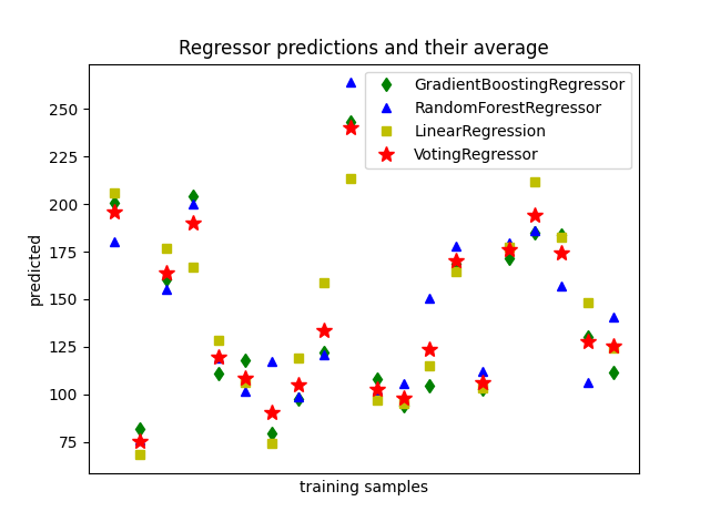
示例
1.11.6. 堆叠概括#
堆叠概括是一种组合估计量以减少其偏差的方法 [W1992] [HTF] .更准确地说,每个独立估计器的预测被堆叠在一起,并用作最终估计器的输入以计算预测。该最终估计器是通过交叉验证训练的。
的 StackingClassifier 和 StackingRegressor 提供可应用于分类和回归问题的策略。
的 estimators 参数对应于输入数据上并行堆叠在一起的估计量列表。它应该作为名称和估计者的列表给出::
>>> from sklearn.linear_model import RidgeCV, LassoCV
>>> from sklearn.neighbors import KNeighborsRegressor
>>> estimators = [('ridge', RidgeCV()),
...               ('lasso', LassoCV(random_state=42)),
...               ('knr', KNeighborsRegressor(n_neighbors=20,
...                                           metric='euclidean'))]
的 final_estimator 将使用 estimators 作为输入。使用时需要是分类器或回归器 StackingClassifier 或 StackingRegressor ,分别::
>>> from sklearn.ensemble import GradientBoostingRegressor
>>> from sklearn.ensemble import StackingRegressor
>>> final_estimator = GradientBoostingRegressor(
...     n_estimators=25, subsample=0.5, min_samples_leaf=25, max_features=1,
...     random_state=42)
>>> reg = StackingRegressor(
...     estimators=estimators,
...     final_estimator=final_estimator)
培养 estimators 和 final_estimator , fit 需要对训练数据调用方法::
>>> from sklearn.datasets import load_diabetes
>>> X, y = load_diabetes(return_X_y=True)
>>> from sklearn.model_selection import train_test_split
>>> X_train, X_test, y_train, y_test = train_test_split(X, y,
...                                                     random_state=42)
>>> reg.fit(X_train, y_train)
StackingRegressor(...)
在训练中, estimators 适合整个训练数据 X_train .打电话时将使用它们 predict 或 predict_proba .为了概括并避免过度贴合, final_estimator 使用外样本进行训练 sklearn.model_selection.cross_val_predict 内部。
为 StackingClassifier ,请注意 estimators 由参数控制 stack_method 它被每个估计器调用。此参数可以是一个字符串(作为估计器方法名称),或者 'auto' 它将根据可用性自动识别可用的方法,并按照偏好顺序进行测试: predict_proba , decision_function 和 predict .
A StackingRegressor 和 StackingClassifier 可以用作任何其他回归器或分类器, predict , predict_proba ,或者 decision_function 方法,例如::
>>> y_pred = reg.predict(X_test)
>>> from sklearn.metrics import r2_score
>>> print('R2 score: {:.2f}'.format(r2_score(y_test, y_pred)))
R2 score: 0.53
请注意,也可以获得堆叠的输出 estimators 使用 transform 方法:
>>> reg.transform(X_test[:5])
array([[142, 138, 146],
       [179, 182, 151],
       [139, 132, 158],
       [286, 292, 225],
       [126, 124, 164]])
在实践中,堆叠预测器的预测效果与基层的最佳预测器一样好,有时甚至通过结合这些预测器的不同优势来优于基层。然而,训练堆叠预测器的计算成本很高。
备注
为 StackingClassifier ,使用时 stack_method_='predict_proba' ,当问题是二元分类问题时,第一列将被删除。事实上,每个估计器预测的两个概率列都完全共线。
备注
通过分配可以实现多个堆叠层 final_estimator 到 StackingClassifier 或 StackingRegressor
>>> final_layer_rfr = RandomForestRegressor(
...     n_estimators=10, max_features=1, max_leaf_nodes=5,random_state=42)
>>> final_layer_gbr = GradientBoostingRegressor(
...     n_estimators=10, max_features=1, max_leaf_nodes=5,random_state=42)
>>> final_layer = StackingRegressor(
...     estimators=[('rf', final_layer_rfr),
...                 ('gbrt', final_layer_gbr)],
...     final_estimator=RidgeCV()
...     )
>>> multi_layer_regressor = StackingRegressor(
...     estimators=[('ridge', RidgeCV()),
...                 ('lasso', LassoCV(random_state=42)),
...                 ('knr', KNeighborsRegressor(n_neighbors=20,
...                                             metric='euclidean'))],
...     final_estimator=final_layer
... )
>>> multi_layer_regressor.fit(X_train, y_train)
StackingRegressor(...)
>>> print('R2 score: {:.2f}'
...       .format(multi_layer_regressor.score(X_test, y_test)))
R2 score: 0.53
示例
引用
作者:David H. "叠加概括。Neural networks 5.2(1992):241 - 259.
1.11.7. AdaBoost#
模块 sklearn.ensemble 包括Freund和Schapire于1995年推出的流行助推算法AdaBoost [FS1995].
AdaBoost的核心原则是适应一系列弱学习者(即,仅比随机猜测稍好的模型,例如小决策树)对重复修改的数据版本。然后,通过加权多数投票(或总和)将所有这些预测组合起来,以产生最终预测。每次所谓的增强迭代中的数据修改都包括应用权重 \(w_1\) , \(w_2\) , ..., \(w_N\) 到每个训练样本。最初,这些权重都设置为 \(w_i = 1/N\) ,因此第一步只是在原始数据上训练弱学习器。对于每个连续的迭代,样本权重被单独修改,并且学习算法被重新应用于重新加权的数据。在给定的步骤中,由在前一步骤中引入的增强模型错误预测的那些训练示例的权重增加,而对于正确预测的那些训练示例的权重减小。随着迭代的进行,难以预测的示例会受到越来越大的影响。因此,每个后续的弱学习者被迫专注于序列中之前的学习者错过的示例 [HTF].

AdaBoost可用于分类和回归问题:
对于多类分类,
AdaBoostClassifier实现AdaBoost. SAME [ZZRH2009].对于回归,
AdaBoostRegressor实现AdaBoost.R2 [D1997].
1.11.7.1. 使用#
下面的示例展示了如何将AdaBoot分类器与100个弱学习者匹配::
>>> from sklearn.model_selection import cross_val_score
>>> from sklearn.datasets import load_iris
>>> from sklearn.ensemble import AdaBoostClassifier

>>> X, y = load_iris(return_X_y=True)
>>> clf = AdaBoostClassifier(n_estimators=100)
>>> scores = cross_val_score(clf, X, y, cv=5)
>>> scores.mean()
np.float64(0.95)
The number of weak learners is controlled by the parameter n_estimators. The
learning_rate parameter controls the contribution of the weak learners in
the final combination. By default, weak learners are decision stumps. Different
weak learners can be specified through the estimator parameter.
The main parameters to tune to obtain good results are n_estimators and
the complexity of the base estimators (e.g., its depth max_depth or
minimum required number of samples to consider a split min_samples_split).
示例
多类AdaBoosted决策树 显示AdaBoost在多类问题上的性能。
两级AdaBoost 显示了使用AdaBoost-SAME的非线性可分两类问题的决策边界和决策函数值。
使用AdaBoost进行决策树回归 演示使用AdaBoost.R2算法的回归。
引用