使用堆叠组合预测因子#

Stacking是一种混合估计量的方法。在这种策略中，一些估计量单独拟合在一些训练数据上，而最终估计量使用这些基本估计量的堆叠预测来训练。

在这个例子中，我们说明了不同的回归量堆叠在一起并使用最终的线性惩罚回归量来输出预测的用例。我们将每个回归量的性能与堆叠策略进行比较。堆叠稍微提高了整体性能。

# Authors: The scikit-learn developers
# SPDX-License-Identifier: BSD-3-Clause

下载数据集#

我们将使用 Ames Housing 该数据集首先由Dean De Cock编制，并在Kaggle挑战中使用后变得更加出名。它是爱荷华州艾姆斯的一套1460套住宅，每套住宅由80个特征描述。我们将使用它来预测房屋的最终对数价格。在这个例子中，我们将仅使用EntityBoostingRegressor（）选择的20个最有趣的功能并限制条目数量（在这里我们不会详细说明如何选择最有趣的功能）。

Ames住房数据集没有随scikit-learn一起提供，因此我们将从 OpenML .

import numpy as np

from sklearn.datasets import fetch_openml
from sklearn.utils import shuffle


def load_ames_housing():
    df = fetch_openml(name="house_prices", as_frame=True)
    X = df.data
    y = df.target

    features = [
        "YrSold",
        "HeatingQC",
        "Street",
        "YearRemodAdd",
        "Heating",
        "MasVnrType",
        "BsmtUnfSF",
        "Foundation",
        "MasVnrArea",
        "MSSubClass",
        "ExterQual",
        "Condition2",
        "GarageCars",
        "GarageType",
        "OverallQual",
        "TotalBsmtSF",
        "BsmtFinSF1",
        "HouseStyle",
        "MiscFeature",
        "MoSold",
    ]

    X = X.loc[:, features]
    X, y = shuffle(X, y, random_state=0)

    X = X.iloc[:600]
    y = y.iloc[:600]
    return X, np.log(y)


X, y = load_ames_housing()

测量并绘制结果#

现在我们可以使用Ames Housing数据集进行预测。我们检查每个单独的预测器以及回归器堆栈的性能。

import time

import matplotlib.pyplot as plt

from sklearn.metrics import PredictionErrorDisplay
from sklearn.model_selection import cross_val_predict, cross_validate

fig, axs = plt.subplots(2, 2, figsize=(9, 7))
axs = np.ravel(axs)

for ax, (name, est) in zip(
    axs, estimators + [("Stacking Regressor", stacking_regressor)]
):
    scorers = {"R2": "r2", "MAE": "neg_mean_absolute_error"}

    start_time = time.time()
    scores = cross_validate(
        est, X, y, scoring=list(scorers.values()), n_jobs=-1, verbose=0
    )
    elapsed_time = time.time() - start_time

    y_pred = cross_val_predict(est, X, y, n_jobs=-1, verbose=0)
    scores = {
        key: (
            f"{np.abs(np.mean(scores[f'test_{value}'])):.2f} +- "
            f"{np.std(scores[f'test_{value}']):.2f}"
        )
        for key, value in scorers.items()
    }

    display = PredictionErrorDisplay.from_predictions(
        y_true=y,
        y_pred=y_pred,
        kind="actual_vs_predicted",
        ax=ax,
        scatter_kwargs={"alpha": 0.2, "color": "tab:blue"},
        line_kwargs={"color": "tab:red"},
    )
    ax.set_title(f"{name}\nEvaluation in {elapsed_time:.2f} seconds")

    for name, score in scores.items():
        ax.plot([], [], " ", label=f"{name}: {score}")
    ax.legend(loc="upper left")

plt.suptitle("Single predictors versus stacked predictors")
plt.tight_layout()
plt.subplots_adjust(top=0.9)
plt.show()

Single predictors versus stacked predictors, Random Forest Evaluation in 1.27 seconds, Lasso Evaluation in 0.30 seconds, Gradient Boosting Evaluation in 0.46 seconds, Stacking Regressor Evaluation in 10.09 seconds

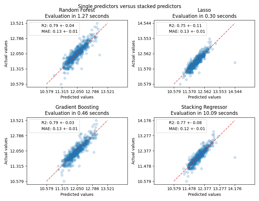
堆叠回归量将结合不同回归量的优势。然而，我们也看到训练堆叠回归量的计算成本要高得多。

Total running time of the script: （0分24.523秒）

使用堆叠组合预测因子#

下载数据集#

制作管道预处理数据#

单个数据集上的预测器堆栈#

测量并绘制结果#