决策树回归#

In this example, we demonstrate the effect of changing the maximum depth of a decision tree on how it fits to the data. We perform this once on a 1D regression task and once on a multi-output regression task.

# Authors: The scikit-learn developers
# SPDX-License-Identifier: BSD-3-Clause

1D回归任务的决策树#

在这里，我们在一维回归任务上拟合一棵树。

的 decision trees 用于在添加噪音观察的情况下匹配sin曲线。结果，它学习逼近sin曲线的局部线性回归。

我们可以看到，如果树的最大深度（由 max_depth 参数）设置得太高，决策树学习训练数据的太细细节并从噪音中学习，即它们过适应。

创建随机1D数据集#

import numpy as np

rng = np.random.RandomState(1)
X = np.sort(5 * rng.rand(80, 1), axis=0)
y = np.sin(X).ravel()
y[::5] += 3 * (0.5 - rng.rand(16))

匹配回归模型#

在这里，我们匹配了两个具有不同最大深度的模型

from sklearn.tree import DecisionTreeRegressor

regr_1 = DecisionTreeRegressor(max_depth=2)
regr_2 = DecisionTreeRegressor(max_depth=5)
regr_1.fit(X, y)
regr_2.fit(X, y)

DecisionTreeRegressor(max_depth=5)

In a Jupyter environment, please rerun this cell to show the HTML representation or trust the notebook.
On GitHub, the HTML representation is unable to render, please try loading this page with nbviewer.org.

预测#

获取测试集的预测

X_test = np.arange(0.0, 5.0, 0.01)[:, np.newaxis]
y_1 = regr_1.predict(X_test)
y_2 = regr_2.predict(X_test)

绘制结果#

import matplotlib.pyplot as plt

plt.figure()
plt.scatter(X, y, s=20, edgecolor="black", c="darkorange", label="data")
plt.plot(X_test, y_1, color="cornflowerblue", label="max_depth=2", linewidth=2)
plt.plot(X_test, y_2, color="yellowgreen", label="max_depth=5", linewidth=2)
plt.xlabel("data")
plt.ylabel("target")
plt.title("Decision Tree Regression")
plt.legend()
plt.show()

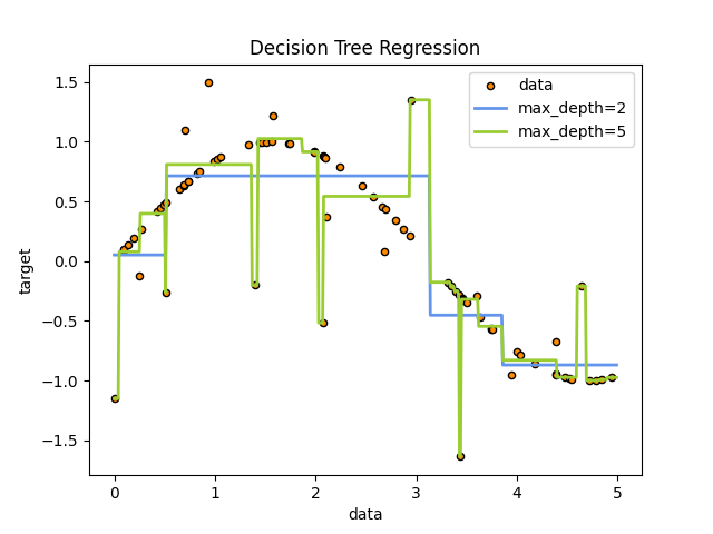
如您所见，深度为5（黄色）的模型学习训练数据的细节，使其过度适合噪音。另一方面，深度为2（蓝色）的模型可以很好地学习数据中的主要趋势，并且不会过度适应。在实际用例中，您需要确保树不会过度适应训练数据，这可以使用交叉验证来完成。

具有多输出目标的决策树回归#

这里 decision trees 用于同时预测噪音 x 和 y 观察一个给定单一基本特征的圆。因此，它学习近似圆的局部线性回归。

我们可以看到，如果树的最大深度（由 max_depth 参数）设置得太高，决策树学习训练数据的太细细节并从噪音中学习，即它们过适应。

创建随机数据集#

rng = np.random.RandomState(1)
X = np.sort(200 * rng.rand(100, 1) - 100, axis=0)
y = np.array([np.pi * np.sin(X).ravel(), np.pi * np.cos(X).ravel()]).T
y[::5, :] += 0.5 - rng.rand(20, 2)

匹配回归模型#

regr_1 = DecisionTreeRegressor(max_depth=2)
regr_2 = DecisionTreeRegressor(max_depth=5)
regr_3 = DecisionTreeRegressor(max_depth=8)
regr_1.fit(X, y)
regr_2.fit(X, y)
regr_3.fit(X, y)

DecisionTreeRegressor(max_depth=8)

In a Jupyter environment, please rerun this cell to show the HTML representation or trust the notebook.
On GitHub, the HTML representation is unable to render, please try loading this page with nbviewer.org.

预测#

获取测试集的预测

X_test = np.arange(-100.0, 100.0, 0.01)[:, np.newaxis]
y_1 = regr_1.predict(X_test)
y_2 = regr_2.predict(X_test)
y_3 = regr_3.predict(X_test)

绘制结果#

plt.figure()
s = 25
plt.scatter(y[:, 0], y[:, 1], c="yellow", s=s, edgecolor="black", label="data")
plt.scatter(
    y_1[:, 0],
    y_1[:, 1],
    c="cornflowerblue",
    s=s,
    edgecolor="black",
    label="max_depth=2",
)
plt.scatter(y_2[:, 0], y_2[:, 1], c="red", s=s, edgecolor="black", label="max_depth=5")
plt.scatter(y_3[:, 0], y_3[:, 1], c="blue", s=s, edgecolor="black", label="max_depth=8")
plt.xlim([-6, 6])
plt.ylim([-6, 6])
plt.xlabel("target 1")
plt.ylabel("target 2")
plt.title("Multi-output Decision Tree Regression")
plt.legend(loc="best")
plt.show()

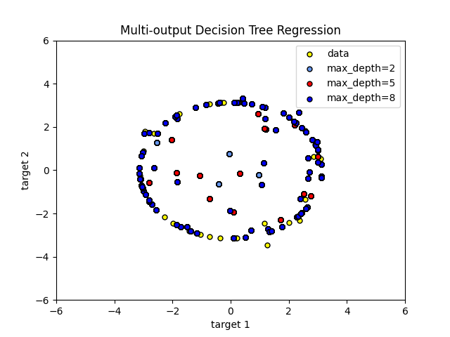
如您所见，的价值越高 max_depth ，模型捕捉到的数据细节就越多。然而，该模型也过度适合数据，并且受到噪音的影响。

Total running time of the script: (0 minutes 0.227 seconds)