Theil-Sen回归#

在合成数据集上计算Theil-Sen回归。

与OLS（普通最小平方）估计器相比，Theil-Sen估计器对异常值具有鲁棒性。在简单线性回归的情况下，它的崩溃点约为29.3%，这意味着在二维情况下，它可以容忍高达29.3%的任意损坏数据（离群值）。

模型的估计是通过计算p个子样本点的所有可能组合的子种群的斜坡和截取来完成的。如果截取已进行匹配，p必须大于或等于n_features + 1。然后将最终的斜坡和相交定义为这些斜坡和相交的空间中位数。

在某些情况下，Theil-Sen的表现优于 RANSAC 这也是一种稳健的方法。这在下面的第二个例子中得到了说明，其中相对于x轴的离群值扰动RASAC。调谐 residual_threshold RASAC的参数弥补了这一点，但一般来说，需要有关数据和异常值性质的先验知识。由于Theil-Sen的计算复杂性，建议仅将其用于样本数量和特征方面的小问题。对于更大的问题， max_subpopulation 参数将p个子样本点的所有可能组合的幅度限制为随机选择的子集，因此也限制了运行时间。因此，Theil-Sen适用于更大的问题，但缺点是失去了一些数学性质，因为它适用于随机子集。

# Authors: The scikit-learn developers
# SPDX-License-Identifier: BSD-3-Clause

import time

import matplotlib.pyplot as plt
import numpy as np

from sklearn.linear_model import LinearRegression, RANSACRegressor, TheilSenRegressor

estimators = [
    ("OLS", LinearRegression()),
    ("Theil-Sen", TheilSenRegressor(random_state=42)),
    ("RANSAC", RANSACRegressor(random_state=42)),
]
colors = {"OLS": "turquoise", "Theil-Sen": "gold", "RANSAC": "lightgreen"}
lw = 2

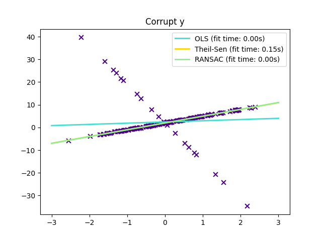
仅在y方向上存在离群值#

np.random.seed(0)
n_samples = 200
# Linear model y = 3*x + N(2, 0.1**2)
x = np.random.randn(n_samples)
w = 3.0
c = 2.0
noise = 0.1 * np.random.randn(n_samples)
y = w * x + c + noise
# 10% outliers
y[-20:] += -20 * x[-20:]
X = x[:, np.newaxis]

plt.scatter(x, y, color="indigo", marker="x", s=40)
line_x = np.array([-3, 3])
for name, estimator in estimators:
    t0 = time.time()
    estimator.fit(X, y)
    elapsed_time = time.time() - t0
    y_pred = estimator.predict(line_x.reshape(2, 1))
    plt.plot(
        line_x,
        y_pred,
        color=colors[name],
        linewidth=lw,
        label="%s (fit time: %.2fs)" % (name, elapsed_time),
    )

plt.axis("tight")
plt.legend(loc="upper right")
_ = plt.title("Corrupt y")

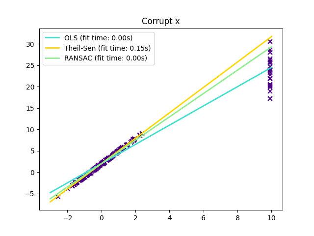
X方向的离群值#

np.random.seed(0)
# Linear model y = 3*x + N(2, 0.1**2)
x = np.random.randn(n_samples)
noise = 0.1 * np.random.randn(n_samples)
y = 3 * x + 2 + noise
# 10% outliers
x[-20:] = 9.9
y[-20:] += 22
X = x[:, np.newaxis]

plt.figure()
plt.scatter(x, y, color="indigo", marker="x", s=40)

line_x = np.array([-3, 10])
for name, estimator in estimators:
    t0 = time.time()
    estimator.fit(X, y)
    elapsed_time = time.time() - t0
    y_pred = estimator.predict(line_x.reshape(2, 1))
    plt.plot(
        line_x,
        y_pred,
        color=colors[name],
        linewidth=lw,
        label="%s (fit time: %.2fs)" % (name, elapsed_time),
    )

plt.axis("tight")
plt.legend(loc="upper left")
plt.title("Corrupt x")
plt.show()

Total running time of the script: （0分0.422秒）