备注

Go to the end 下载完整的示例代码。或者通过浏览器中的MysterLite或Binder运行此示例

Faces数据集分解#

这个例子适用于奥利韦蒂面临数据集模块中不同的无监督矩阵分解（降维）方法 sklearn.decomposition (see文档章节将信号分解为分量（矩阵分解问题） ).

# Authors: The scikit-learn developers
# SPDX-License-Identifier: BSD-3-Clause

数据集准备#

加载和预处理Olivetti面部数据集。

import logging

import matplotlib.pyplot as plt
from numpy.random import RandomState

from sklearn import cluster, decomposition
from sklearn.datasets import fetch_olivetti_faces

rng = RandomState(0)

# Display progress logs on stdout
logging.basicConfig(level=logging.INFO, format="%(asctime)s %(levelname)s %(message)s")

faces, _ = fetch_olivetti_faces(return_X_y=True, shuffle=True, random_state=rng)
n_samples, n_features = faces.shape

# Global centering (focus on one feature, centering all samples)
faces_centered = faces - faces.mean(axis=0)

# Local centering (focus on one sample, centering all features)
faces_centered -= faces_centered.mean(axis=1).reshape(n_samples, -1)

print("Dataset consists of %d faces" % n_samples)

Dataset consists of 400 faces

定义基本函数来绘制面库。

n_row, n_col = 2, 3
n_components = n_row * n_col
image_shape = (64, 64)


def plot_gallery(title, images, n_col=n_col, n_row=n_row, cmap=plt.cm.gray):
    fig, axs = plt.subplots(
        nrows=n_row,
        ncols=n_col,
        figsize=(2.0 * n_col, 2.3 * n_row),
        facecolor="white",
        constrained_layout=True,
    )
    fig.set_constrained_layout_pads(w_pad=0.01, h_pad=0.02, hspace=0, wspace=0)
    fig.set_edgecolor("black")
    fig.suptitle(title, size=16)
    for ax, vec in zip(axs.flat, images):
        vmax = max(vec.max(), -vec.min())
        im = ax.imshow(
            vec.reshape(image_shape),
            cmap=cmap,
            interpolation="nearest",
            vmin=-vmax,
            vmax=vmax,
        )
        ax.axis("off")

    fig.colorbar(im, ax=axs, orientation="horizontal", shrink=0.99, aspect=40, pad=0.01)
    plt.show()

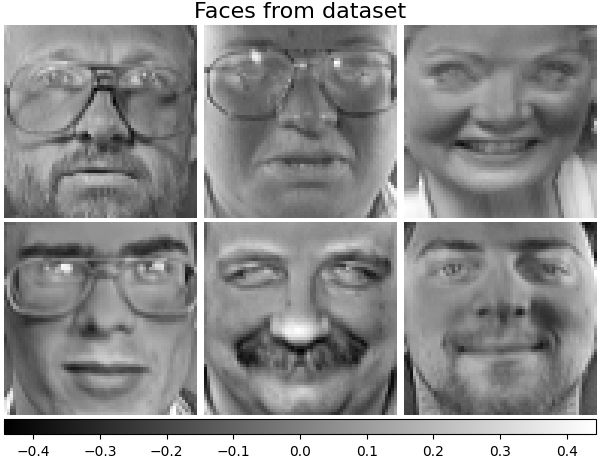
让我们看看我们的数据。灰色表示负值，白色表示正值。

plot_gallery("Faces from dataset", faces_centered[:n_components])

分解#

初始化不同的估计器进行分解，并将每个估计器匹配到所有图像上并绘制一些结果。每个估计器提取6个分量作为载体 \(h \in \mathbb{R}^{4096}\) .我们只是以人性友好的可视化方式将这些载体显示为64 x64像素图像。

阅读更多的 User Guide .

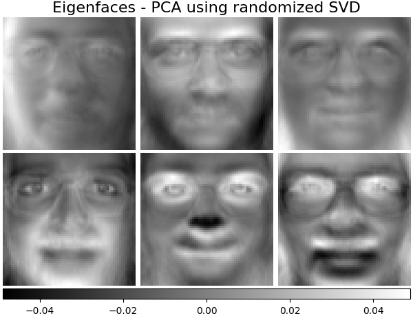
特征面-使用随机奇异值分解的PCA#

使用数据的奇异值分解（DID）进行线性降维，将其投影到较低维空间。

备注

Eigenfaces估计器，通过 sklearn.decomposition.PCA ，还提供了一个纯量 noise_variance_ (the像素方差的平均值），无法显示为图像。

pca_estimator = decomposition.PCA(
    n_components=n_components, svd_solver="randomized", whiten=True
)
pca_estimator.fit(faces_centered)
plot_gallery(
    "Eigenfaces - PCA using randomized SVD", pca_estimator.components_[:n_components]
)

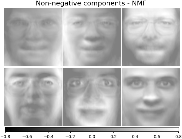
非负成分- NMF#

将非负原始数据估计为两个非负矩阵的产生。

nmf_estimator = decomposition.NMF(n_components=n_components, tol=5e-3)
nmf_estimator.fit(faces)  # original non- negative dataset
plot_gallery("Non-negative components - NMF", nmf_estimator.components_[:n_components])

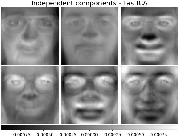
独立组件- FastICA#

独立分量分析将多变量向量分离成最大独立的可加子分量。

ica_estimator = decomposition.FastICA(
    n_components=n_components, max_iter=400, whiten="arbitrary-variance", tol=15e-5
)
ica_estimator.fit(faces_centered)
plot_gallery(
    "Independent components - FastICA", ica_estimator.components_[:n_components]
)

稀疏组件- MiniBatchSparsePCA#

小批量稀疏PCA (MiniBatchSparsePCA ）提取最佳重构数据的稀疏分量的集合。这种变体比类似的更快，但准确性较差。 SparsePCA .

batch_pca_estimator = decomposition.MiniBatchSparsePCA(
    n_components=n_components, alpha=0.1, max_iter=100, batch_size=3, random_state=rng
)
batch_pca_estimator.fit(faces_centered)
plot_gallery(
    "Sparse components - MiniBatchSparsePCA",
    batch_pca_estimator.components_[:n_components],
)

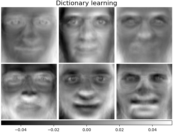
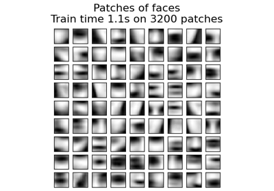
字典学习#

默认情况下， MiniBatchDictionaryLearning 将数据分为小批，并通过循环小批指定迭代次数来以在线方式进行优化。

batch_dict_estimator = decomposition.MiniBatchDictionaryLearning(
    n_components=n_components, alpha=0.1, max_iter=50, batch_size=3, random_state=rng
)
batch_dict_estimator.fit(faces_centered)
plot_gallery("Dictionary learning", batch_dict_estimator.components_[:n_components])

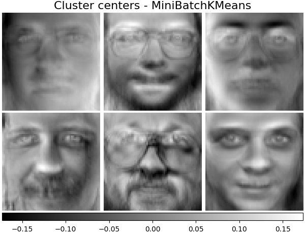
集群中心- MiniBatchKMeans#

sklearn.cluster.MiniBatchKMeans 是计算效率和实现在线学习与 partial_fit 法这就是为什么通过以下方式增强一些耗时的算法可能是有益的 MiniBatchKMeans .

kmeans_estimator = cluster.MiniBatchKMeans(
    n_clusters=n_components,
    tol=1e-3,
    batch_size=20,
    max_iter=50,
    random_state=rng,
)
kmeans_estimator.fit(faces_centered)
plot_gallery(
    "Cluster centers - MiniBatchKMeans",
    kmeans_estimator.cluster_centers_[:n_components],
)

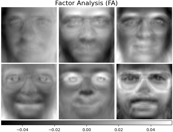
因子分析组件- FA#

FactorAnalysis 类似于 PCA 但是具有独立地对输入空间的每个方向上的方差（异方差噪声）进行建模的优点。阅读更多的 User Guide .

fa_estimator = decomposition.FactorAnalysis(n_components=n_components, max_iter=20)
fa_estimator.fit(faces_centered)
plot_gallery("Factor Analysis (FA)", fa_estimator.components_[:n_components])

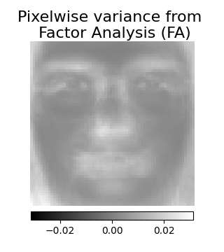
# --- Pixelwise variance
plt.figure(figsize=(3.2, 3.6), facecolor="white", tight_layout=True)
vec = fa_estimator.noise_variance_
vmax = max(vec.max(), -vec.min())
plt.imshow(
    vec.reshape(image_shape),
    cmap=plt.cm.gray,
    interpolation="nearest",
    vmin=-vmax,
    vmax=vmax,
)
plt.axis("off")
plt.title("Pixelwise variance from \n Factor Analysis (FA)", size=16, wrap=True)
plt.colorbar(orientation="horizontal", shrink=0.8, pad=0.03)
plt.show()

分解：词典学习#

在下一部分中，让我们考虑一下字典学习更准确地说。字典学习是一个问题，相当于将输入数据的稀疏表示作为简单元素的组合。这些简单的元素构成了一本字典。可以将字典和/或编码系数约束为正，以匹配数据中可能存在的约束。

MiniBatchDictionaryLearning 实现了更快、但不太准确的字典学习算法版本，该算法更适合大型数据集。阅读更多的 User Guide .

从我们的数据集中绘制相同的样本，但使用另一个颜色图。红色表示负值，蓝色表示正值，白色表示零。

plot_gallery("Faces from dataset", faces_centered[:n_components], cmap=plt.cm.RdBu)

Similar to the previous examples, we change parameters and train MiniBatchDictionaryLearning estimator on all images. Generally, the dictionary learning and sparse encoding decompose input data into the dictionary and the coding coefficients matrices. \(X \approx UV\), where \(X = [x_1, . . . , x_n]\), \(X \in \mathbb{R}^{m×n}\), dictionary \(U \in \mathbb{R}^{m×k}\), coding coefficients \(V \in \mathbb{R}^{k×n}\).

下面还列出了字典和编码系数受到正约束时的结果。

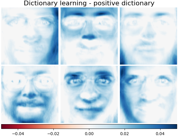
词典学习-积极词典#

在下一节中，我们在查找字典时强制采取积极态度。

dict_pos_dict_estimator = decomposition.MiniBatchDictionaryLearning(
    n_components=n_components,
    alpha=0.1,
    max_iter=50,
    batch_size=3,
    random_state=rng,
    positive_dict=True,
)
dict_pos_dict_estimator.fit(faces_centered)
plot_gallery(
    "Dictionary learning - positive dictionary",
    dict_pos_dict_estimator.components_[:n_components],
    cmap=plt.cm.RdBu,
)

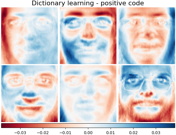
Dictionary learning - positive dictionary

字典学习-正代码#

下面我们将编码系数约束为正矩阵。

dict_pos_code_estimator = decomposition.MiniBatchDictionaryLearning(
    n_components=n_components,
    alpha=0.1,
    max_iter=50,
    batch_size=3,
    fit_algorithm="cd",
    random_state=rng,
    positive_code=True,
)
dict_pos_code_estimator.fit(faces_centered)
plot_gallery(
    "Dictionary learning - positive code",
    dict_pos_code_estimator.components_[:n_components],
    cmap=plt.cm.RdBu,
)

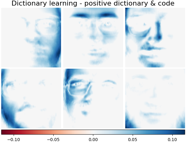
词典学习-积极的词典和代码#

下面还列出了字典值和编码系数受到正约束的结果。

dict_pos_estimator = decomposition.MiniBatchDictionaryLearning(
    n_components=n_components,
    alpha=0.1,
    max_iter=50,
    batch_size=3,
    fit_algorithm="cd",
    random_state=rng,
    positive_dict=True,
    positive_code=True,
)
dict_pos_estimator.fit(faces_centered)
plot_gallery(
    "Dictionary learning - positive dictionary & code",
    dict_pos_estimator.components_[:n_components],
    cmap=plt.cm.RdBu,
)

Dictionary learning - positive dictionary & code

Total running time of the script: （0分7.421秒）