基于模型的顺序特征选择#

本示例说明并比较了两种特征选择方法： SelectFromModel 这基于特征重要性，并且 SequentialFeatureSelector 这依赖于贪婪的方法。

我们使用糖尿病数据集，该数据集由从442名糖尿病患者收集的10个特征组成。

# Authors: The scikit-learn developers
# SPDX-License-Identifier: BSD-3-Clause

加载数据#

我们首先加载可从scikit-learn中获取的糖尿病数据集，并打印其描述：

from sklearn.datasets import load_diabetes

diabetes = load_diabetes()
X, y = diabetes.data, diabetes.target
print(diabetes.DESCR)

.. _diabetes_dataset:

Diabetes dataset
----------------

Ten baseline variables, age, sex, body mass index, average blood
pressure, and six blood serum measurements were obtained for each of n =
442 diabetes patients, as well as the response of interest, a
quantitative measure of disease progression one year after baseline.

**Data Set Characteristics:**

:Number of Instances: 442

:Number of Attributes: First 10 columns are numeric predictive values

:Target: Column 11 is a quantitative measure of disease progression one year after baseline

:Attribute Information:
    - age     age in years
    - sex
    - bmi     body mass index
    - bp      average blood pressure
    - s1      tc, total serum cholesterol
    - s2      ldl, low-density lipoproteins
    - s3      hdl, high-density lipoproteins
    - s4      tch, total cholesterol / HDL
    - s5      ltg, possibly log of serum triglycerides level
    - s6      glu, blood sugar level

Note: Each of these 10 feature variables have been mean centered and scaled by the standard deviation times the square root of `n_samples` (i.e. the sum of squares of each column totals 1).

Source URL:
https://www4.stat.ncsu.edu/~boos/var.select/diabetes.html

For more information see:
Bradley Efron, Trevor Hastie, Iain Johnstone and Robert Tibshirani (2004) "Least Angle Regression," Annals of Statistics (with discussion), 407-499.
(https://web.stanford.edu/~hastie/Papers/LARS/LeastAngle_2002.pdf)

来自系数的特征重要性#

为了了解这些功能的重要性，我们将使用 RidgeCV 估计者。具有最高绝对值的特征 coef_ 价值被认为是最重要的。我们可以直接观察系数，而无需缩放它们（或缩放数据），因为从上面的描述中，我们知道这些特征已经标准化了。有关线性模型系数解释的更完整示例，您可以参考线性模型系数解释中的常见陷阱 . # noqa：E501

import matplotlib.pyplot as plt
import numpy as np

from sklearn.linear_model import RidgeCV

ridge = RidgeCV(alphas=np.logspace(-6, 6, num=5)).fit(X, y)
importance = np.abs(ridge.coef_)
feature_names = np.array(diabetes.feature_names)
plt.bar(height=importance, x=feature_names)
plt.title("Feature importances via coefficients")
plt.show()

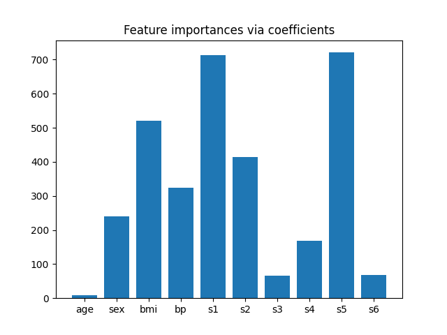
根据重要性选择要素#

现在我们要根据系数选择最重要的两个特征。的 SelectFromModel 就是为了这个。 SelectFromModel 接受一个 threshold 参数并将选择重要性（由系数定义）高于此阈值的特征。

由于我们只想选择2个特征，我们将这个阈值设置为略高于第三重要特征的系数。

from time import time

from sklearn.feature_selection import SelectFromModel

threshold = np.sort(importance)[-3] + 0.01

tic = time()
sfm = SelectFromModel(ridge, threshold=threshold).fit(X, y)
toc = time()
print(f"Features selected by SelectFromModel: {feature_names[sfm.get_support()]}")
print(f"Done in {toc - tic:.3f}s")

Features selected by SelectFromModel: ['s1' 's5']
Done in 0.002s

通过顺序特征选择选择特征#

选择要素的另一种方法是使用 SequentialFeatureSelector （SFS）。SFS是一个贪婪的过程，在每次迭代时，我们都会根据交叉验证分数选择最佳的新功能添加到我们所选的功能中。也就是说，我们从0个功能开始，选择得分最高的最佳单个功能。重复该过程，直到达到所需的选定特征数量。

我们还可以反向（向后SFS）， i.e. 从所有功能开始，贪婪地选择要逐个删除的功能。我们在这里说明了这两种方法。

from sklearn.feature_selection import SequentialFeatureSelector

tic_fwd = time()
sfs_forward = SequentialFeatureSelector(
    ridge, n_features_to_select=2, direction="forward"
).fit(X, y)
toc_fwd = time()

tic_bwd = time()
sfs_backward = SequentialFeatureSelector(
    ridge, n_features_to_select=2, direction="backward"
).fit(X, y)
toc_bwd = time()

print(
    "Features selected by forward sequential selection: "
    f"{feature_names[sfs_forward.get_support()]}"
)
print(f"Done in {toc_fwd - tic_fwd:.3f}s")
print(
    "Features selected by backward sequential selection: "
    f"{feature_names[sfs_backward.get_support()]}"
)
print(f"Done in {toc_bwd - tic_bwd:.3f}s")

Features selected by forward sequential selection: ['bmi' 's5']
Done in 0.181s
Features selected by backward sequential selection: ['bmi' 's5']
Done in 0.476s

有趣的是，向前和向后选择选择了相同的特征集。一般来说，情况并非如此，两种方法会导致不同的结果。

我们还注意到，SFS选择的功能与通过功能重要性选择的功能不同：SFS选择 bmi 而不是 s1 .但这听起来确实合理，因为 bmi 根据系数，对应于第三重要的特征。考虑到SFS根本没有使用系数，这是相当值得注意的。

最后，我们应该注意到 SelectFromModel 比SFS快得多。事实上， SelectFromModel 只需对模型进行一次匹配，而SFS需要为每次迭代交叉验证许多不同的模型。然而，SFS适用于任何模型，而 SelectFromModel 要求基础估计器暴露 coef_ 属性或 feature_importances_ 属性向前SFS比向后SFS更快，因为它只需要执行 n_features_to_select = 2 迭代，而向后SFS需要执行 n_features - n_features_to_select = 8 迭代。

使用负容差值#

SequentialFeatureSelector 可用于删除数据集中存在的要素并返回原始要素的较小子集 direction="backward" 和负值 tol .

我们首先加载乳腺癌数据集，该数据集由30个不同的特征和569个样本组成。

import numpy as np

from sklearn.datasets import load_breast_cancer

breast_cancer_data = load_breast_cancer()
X, y = breast_cancer_data.data, breast_cancer_data.target
feature_names = np.array(breast_cancer_data.feature_names)
print(breast_cancer_data.DESCR)

.. _breast_cancer_dataset:

Breast cancer wisconsin (diagnostic) dataset
--------------------------------------------

**Data Set Characteristics:**

:Number of Instances: 569

:Number of Attributes: 30 numeric, predictive attributes and the class

:Attribute Information:
    - radius (mean of distances from center to points on the perimeter)
    - texture (standard deviation of gray-scale values)
    - perimeter
    - area
    - smoothness (local variation in radius lengths)
    - compactness (perimeter^2 / area - 1.0)
    - concavity (severity of concave portions of the contour)
    - concave points (number of concave portions of the contour)
    - symmetry
    - fractal dimension ("coastline approximation" - 1)

    The mean, standard error, and "worst" or largest (mean of the three
    worst/largest values) of these features were computed for each image,
    resulting in 30 features.  For instance, field 0 is Mean Radius, field
    10 is Radius SE, field 20 is Worst Radius.

    - class:
            - WDBC-Malignant
            - WDBC-Benign

:Summary Statistics:

===================================== ====== ======
                                        Min    Max
===================================== ====== ======
radius (mean):                        6.981  28.11
texture (mean):                       9.71   39.28
perimeter (mean):                     43.79  188.5
area (mean):                          143.5  2501.0
smoothness (mean):                    0.053  0.163
compactness (mean):                   0.019  0.345
concavity (mean):                     0.0    0.427
concave points (mean):                0.0    0.201
symmetry (mean):                      0.106  0.304
fractal dimension (mean):             0.05   0.097
radius (standard error):              0.112  2.873
texture (standard error):             0.36   4.885
perimeter (standard error):           0.757  21.98
area (standard error):                6.802  542.2
smoothness (standard error):          0.002  0.031
compactness (standard error):         0.002  0.135
concavity (standard error):           0.0    0.396
concave points (standard error):      0.0    0.053
symmetry (standard error):            0.008  0.079
fractal dimension (standard error):   0.001  0.03
radius (worst):                       7.93   36.04
texture (worst):                      12.02  49.54
perimeter (worst):                    50.41  251.2
area (worst):                         185.2  4254.0
smoothness (worst):                   0.071  0.223
compactness (worst):                  0.027  1.058
concavity (worst):                    0.0    1.252
concave points (worst):               0.0    0.291
symmetry (worst):                     0.156  0.664
fractal dimension (worst):            0.055  0.208
===================================== ====== ======

:Missing Attribute Values: None

:Class Distribution: 212 - Malignant, 357 - Benign

:Creator:  Dr. William H. Wolberg, W. Nick Street, Olvi L. Mangasarian

:Donor: Nick Street

:Date: November, 1995

This is a copy of UCI ML Breast Cancer Wisconsin (Diagnostic) datasets.
https://goo.gl/U2Uwz2

Features are computed from a digitized image of a fine needle
aspirate (FNA) of a breast mass.  They describe
characteristics of the cell nuclei present in the image.

Separating plane described above was obtained using
Multisurface Method-Tree (MSM-T) [K. P. Bennett, "Decision Tree
Construction Via Linear Programming." Proceedings of the 4th
Midwest Artificial Intelligence and Cognitive Science Society,
pp. 97-101, 1992], a classification method which uses linear
programming to construct a decision tree.  Relevant features
were selected using an exhaustive search in the space of 1-4
features and 1-3 separating planes.

The actual linear program used to obtain the separating plane
in the 3-dimensional space is that described in:
[K. P. Bennett and O. L. Mangasarian: "Robust Linear
Programming Discrimination of Two Linearly Inseparable Sets",
Optimization Methods and Software 1, 1992, 23-34].

This database is also available through the UW CS ftp server:

ftp ftp.cs.wisc.edu
cd math-prog/cpo-dataset/machine-learn/WDBC/

.. dropdown:: References

  - W.N. Street, W.H. Wolberg and O.L. Mangasarian. Nuclear feature extraction
    for breast tumor diagnosis. IS&T/SPIE 1993 International Symposium on
    Electronic Imaging: Science and Technology, volume 1905, pages 861-870,
    San Jose, CA, 1993.
  - O.L. Mangasarian, W.N. Street and W.H. Wolberg. Breast cancer diagnosis and
    prognosis via linear programming. Operations Research, 43(4), pages 570-577,
    July-August 1995.
  - W.H. Wolberg, W.N. Street, and O.L. Mangasarian. Machine learning techniques
    to diagnose breast cancer from fine-needle aspirates. Cancer Letters 77 (1994)
    163-171.

We will make use of the LogisticRegression estimator with SequentialFeatureSelector to perform the feature selection.

from sklearn.linear_model import LogisticRegression
from sklearn.metrics import roc_auc_score
from sklearn.pipeline import make_pipeline
from sklearn.preprocessing import StandardScaler

for tol in [-1e-2, -1e-3, -1e-4]:
    start = time()
    feature_selector = SequentialFeatureSelector(
        LogisticRegression(),
        n_features_to_select="auto",
        direction="backward",
        scoring="roc_auc",
        tol=tol,
        n_jobs=2,
    )
    model = make_pipeline(StandardScaler(), feature_selector, LogisticRegression())
    model.fit(X, y)
    end = time()
    print(f"\ntol: {tol}")
    print(f"Features selected: {feature_names[model[1].get_support()]}")
    print(f"ROC AUC score: {roc_auc_score(y, model.predict_proba(X)[:, 1]):.3f}")
    print(f"Done in {end - start:.3f}s")

tol: -0.01
Features selected: ['worst perimeter']
ROC AUC score: 0.975
Done in 10.794s

tol: -0.001
Features selected: ['radius error' 'fractal dimension error' 'worst texture'
 'worst perimeter' 'worst concave points']
ROC AUC score: 0.997
Done in 10.772s

tol: -0.0001
Features selected: ['mean compactness' 'mean concavity' 'mean concave points' 'radius error'
 'area error' 'concave points error' 'symmetry error'
 'fractal dimension error' 'worst texture' 'worst perimeter' 'worst area'
 'worst concave points' 'worst symmetry']
ROC AUC score: 0.998
Done in 8.933s

我们可以看到，选择的特征数量往往会随着负值而增加 tol 接近零。随着 tol 接近于零。

Total running time of the script: （0分31.233秒）