备注
Go to the end 下载完整的示例代码。或者通过浏览器中的MysterLite或Binder运行此示例
收件箱Hasher和DictVectorizer比较#
在这个例子中,我们说明了文本载体化,这是将非数字输入数据(例如字典或文本文档)表示为真实数字的载体的过程。
我们首先比较 FeatureHasher 和 DictVectorizer 通过使用这两种方法来对在自定义Python函数的帮助下进行预处理(标记化)的文本文档进行载体化。
稍后我们介绍并分析特定于文本的载体器 HashingVectorizer , CountVectorizer 和 TfidfVectorizer 它处理符号化和特征矩阵在单个类内的组装。
该示例的目的是演示文本载体化API的使用并比较它们的处理时间。查看示例脚本 使用稀疏特征对文本文档进行分类 和 基于k-means的文本聚类 用于实际学习文本文档。
# Authors: The scikit-learn developers
# SPDX-License-Identifier: BSD-3-Clause
加载数据#
我们从 20个新闻组文本数据集 ,其中包括约18000个新闻组帖子,涉及20个主题,分为两个子集:一个用于培训,一个用于测试。为了简单起见并降低计算成本,我们选择了7个主题的子集并仅使用训练集。
from sklearn.datasets import fetch_20newsgroups

categories = [
    "alt.atheism",
    "comp.graphics",
    "comp.sys.ibm.pc.hardware",
    "misc.forsale",
    "rec.autos",
    "sci.space",
    "talk.religion.misc",
]

print("Loading 20 newsgroups training data")
raw_data, _ = fetch_20newsgroups(subset="train", categories=categories, return_X_y=True)
data_size_mb = sum(len(s.encode("utf-8")) for s in raw_data) / 1e6
print(f"{len(raw_data)} documents - {data_size_mb:.3f}MB")
Loading 20 newsgroups training data
3803 documents - 6.245MB
定义预处理功能#
标记可以是一个单词、单词的一部分或字符串中的空白或符号之间包含的任何内容。在这里,我们定义了一个函数,该函数使用匹配Unicode单词字符的简单正规表达(regex)提取标记。这包括任何语言中可以成为单词一部分的大多数字符,以及数字和强调线:
import re


def tokenize(doc):
    """Extract tokens from doc.

    This uses a simple regex that matches word characters to break strings
    into tokens. For a more principled approach, see CountVectorizer or
    TfidfVectorizer.
    """
    return (tok.lower() for tok in re.findall(r"\w+", doc))


list(tokenize("This is a simple example, isn't it?"))
['this', 'is', 'a', 'simple', 'example', 'isn', 't', 'it']
我们定义了一个额外的函数,该函数计算给定文档中每个标记的出现频率。它返回一个要由载体使用的频率字典。
from collections import defaultdict


def token_freqs(doc):
    """Extract a dict mapping tokens from doc to their occurrences."""

    freq = defaultdict(int)
    for tok in tokenize(doc):
        freq[tok] += 1
    return freq


token_freqs("That is one example, but this is another one")
defaultdict(<class 'int'>, {'that': 1, 'is': 2, 'one': 2, 'example': 1, 'but': 1, 'this': 1, 'another': 1})
特别注意重复的记号 "is" 例如,被计数两次。
将文本文档分解为单词标记,可能会丢失句子中单词之间的顺序信息通常称为 Bag of Words representation .
DictVectorizer#
首先我们对 DictVectorizer ,然后我们将其与 FeatureHasher 因为它们都接收词典作为输入。
from time import time

from sklearn.feature_extraction import DictVectorizer

dict_count_vectorizers = defaultdict(list)

t0 = time()
vectorizer = DictVectorizer()
vectorizer.fit_transform(token_freqs(d) for d in raw_data)
duration = time() - t0
dict_count_vectorizers["vectorizer"].append(
    vectorizer.__class__.__name__ + "\non freq dicts"
)
dict_count_vectorizers["speed"].append(data_size_mb / duration)
print(f"done in {duration:.3f} s at {data_size_mb / duration:.1f} MB/s")
print(f"Found {len(vectorizer.get_feature_names_out())} unique terms")
done in 0.691 s at 9.0 MB/s
Found 47928 unique terms
从文本标记到列索引的实际映射显式存储在 .vocabulary_ 属性,这可能是一个非常大的Python字典:
type(vectorizer.vocabulary_)
len(vectorizer.vocabulary_)
47928
vectorizer.vocabulary_["example"]
19145
FeatureHasher#
随着训练集的增长,词典会占用大量的存储空间,并且大小也会增加。特征哈希不是与字典一起增长,而是通过应用哈希函数来构建预定义长度的载体 h 对于特征(例如,令牌),然后直接使用散列值作为特征索引,并在这些索引处更新结果向量。当特征空间不够大时,散列函数往往会将不同的值映射到相同的散列代码(散列冲突)。因此,不可能确定是什么对象生成了任何特定的哈希代码。
由于上述原因,不可能从特征矩阵中恢复原始令牌,并且估计原始字典中唯一词条数量的最佳方法是计算编码特征矩阵中活动列的数量。为此目的,我们定义了以下函数:
import numpy as np


def n_nonzero_columns(X):
    """Number of columns with at least one non-zero value in a CSR matrix.

    This is useful to count the number of features columns that are effectively
    active when using the FeatureHasher.
    """
    return len(np.unique(X.nonzero()[1]))
的默认功能数 FeatureHasher 为2 20. Here we set `n_features = 2 18 '来说明哈希冲突。
FeatureHasher on frequency dictionaries
from sklearn.feature_extraction import FeatureHasher

t0 = time()
hasher = FeatureHasher(n_features=2**18)
X = hasher.transform(token_freqs(d) for d in raw_data)
duration = time() - t0
dict_count_vectorizers["vectorizer"].append(
    hasher.__class__.__name__ + "\non freq dicts"
)
dict_count_vectorizers["speed"].append(data_size_mb / duration)
print(f"done in {duration:.3f} s at {data_size_mb / duration:.1f} MB/s")
print(f"Found {n_nonzero_columns(X)} unique tokens")
done in 0.429 s at 14.6 MB/s
Found 43873 unique tokens
使用时唯一令牌的数量 FeatureHasher 低于使用 DictVectorizer .这是由于哈希冲突造成的。
可以通过增加特征空间来减少碰撞的数量。请注意,当设置大量特征时,向量器的速度不会显着变化,尽管它会导致更大的系数维度,然后需要更多的内存使用来存储它们,即使其中大部分是不活动的。
t0 = time()
hasher = FeatureHasher(n_features=2**22)
X = hasher.transform(token_freqs(d) for d in raw_data)
duration = time() - t0

print(f"done in {duration:.3f} s at {data_size_mb / duration:.1f} MB/s")
print(f"Found {n_nonzero_columns(X)} unique tokens")
done in 0.428 s at 14.6 MB/s
Found 47668 unique tokens
我们确认唯一代币的数量越来越接近 DictVectorizer .
FeatureHasher on raw tokens
或者,可以设置 input_type="string" 在 FeatureHasher 将直接从自定义的输出的字符串进行垂直化 tokenize 功能这相当于为每个要素名称传递隐含频率为1的字典。
t0 = time()
hasher = FeatureHasher(n_features=2**18, input_type="string")
X = hasher.transform(tokenize(d) for d in raw_data)
duration = time() - t0
dict_count_vectorizers["vectorizer"].append(
    hasher.__class__.__name__ + "\non raw tokens"
)
dict_count_vectorizers["speed"].append(data_size_mb / duration)
print(f"done in {duration:.3f} s at {data_size_mb / duration:.1f} MB/s")
print(f"Found {n_nonzero_columns(X)} unique tokens")
done in 0.406 s at 15.4 MB/s
Found 43873 unique tokens
现在我们绘制上述方法进行载体化的速度。
import matplotlib.pyplot as plt

fig, ax = plt.subplots(figsize=(12, 6))

y_pos = np.arange(len(dict_count_vectorizers["vectorizer"]))
ax.barh(y_pos, dict_count_vectorizers["speed"], align="center")
ax.set_yticks(y_pos)
ax.set_yticklabels(dict_count_vectorizers["vectorizer"])
ax.invert_yaxis()
_ = ax.set_xlabel("speed (MB/s)")
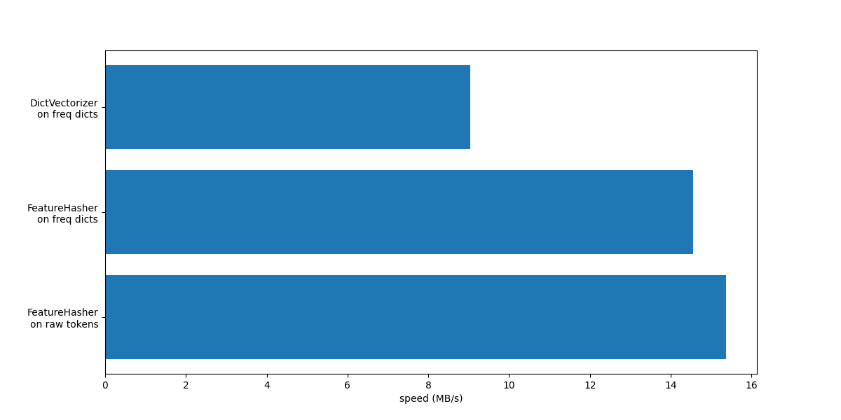
在这两种情况下 FeatureHasher 速度大约是两倍 DictVectorizer .这在处理大量数据时很方便,但缺点是失去转换的可逆性,这反过来又使模型的解释成为一项更加复杂的任务。
的 FeatureHeasher 与 input_type="string" 比适用于频率dict的变体稍快,因为它不计算重复的令牌:每个令牌隐式计数一次,即使它是重复的。根据下游机器学习任务的不同,这可能是一种限制。
与专用文本矢量化工具的比较#
CountVectorizer 接受原始数据,因为它在内部实施标记化和发生计数。它类似于 DictVectorizer 与定制功能一起使用时 token_freqs 正如上一节所做的那样。区别在于 CountVectorizer 更加灵活。特别是,它通过 token_pattern 参数.
from sklearn.feature_extraction.text import CountVectorizer

t0 = time()
vectorizer = CountVectorizer()
vectorizer.fit_transform(raw_data)
duration = time() - t0
dict_count_vectorizers["vectorizer"].append(vectorizer.__class__.__name__)
dict_count_vectorizers["speed"].append(data_size_mb / duration)
print(f"done in {duration:.3f} s at {data_size_mb / duration:.1f} MB/s")
print(f"Found {len(vectorizer.get_feature_names_out())} unique terms")
done in 0.445 s at 14.0 MB/s
Found 47885 unique terms
We see that using the CountVectorizer
implementation is approximately twice as fast as using the
DictVectorizer along with the simple
function we defined for mapping the tokens. The reason is that
CountVectorizer is optimized by
reusing a compiled regular expression for the full training set instead of
creating one per document as done in our naive tokenize function.
现在我们用 HashingVectorizer ,相当于结合了 FeatureHasher 类以及 CountVectorizer .
from sklearn.feature_extraction.text import HashingVectorizer

t0 = time()
vectorizer = HashingVectorizer(n_features=2**18)
vectorizer.fit_transform(raw_data)
duration = time() - t0
dict_count_vectorizers["vectorizer"].append(vectorizer.__class__.__name__)
dict_count_vectorizers["speed"].append(data_size_mb / duration)
print(f"done in {duration:.3f} s at {data_size_mb / duration:.1f} MB/s")
done in 0.342 s at 18.3 MB/s
我们可以观察到,这是迄今为止最快的文本标记化策略,假设下游机器学习任务可以容忍一些冲突。
TfidfVectorizer#
在大型文本库中,某些单词出现的频率较高(例如英语中的“the”、“a”、“is”),并且不携带有关文档实际内容的有意义的信息。如果我们将字数数据直接提供给分类器,那么这些非常常见的术语将掩盖更罕见但信息量更大的术语的频率。为了将计数特征重新加权为适合分类器使用的浮点值,使用由 TfidfTransformer . TF代表“术语频率”,而“tf-idf”意味着术语频率乘以逆文档频率。
我们现在对 TfidfVectorizer ,相当于将 CountVectorizer 以及来自a的标准化和加权 TfidfTransformer .
from sklearn.feature_extraction.text import TfidfVectorizer

t0 = time()
vectorizer = TfidfVectorizer()
vectorizer.fit_transform(raw_data)
duration = time() - t0
dict_count_vectorizers["vectorizer"].append(vectorizer.__class__.__name__)
dict_count_vectorizers["speed"].append(data_size_mb / duration)
print(f"done in {duration:.3f} s at {data_size_mb / duration:.1f} MB/s")
print(f"Found {len(vectorizer.get_feature_names_out())} unique terms")
done in 0.451 s at 13.8 MB/s
Found 47885 unique terms
总结#
让我们通过在单个图中总结所有记录的处理速度来结束本笔记本:
fig, ax = plt.subplots(figsize=(12, 6))

y_pos = np.arange(len(dict_count_vectorizers["vectorizer"]))
ax.barh(y_pos, dict_count_vectorizers["speed"], align="center")
ax.set_yticks(y_pos)
ax.set_yticklabels(dict_count_vectorizers["vectorizer"])
ax.invert_yaxis()
_ = ax.set_xlabel("speed (MB/s)")
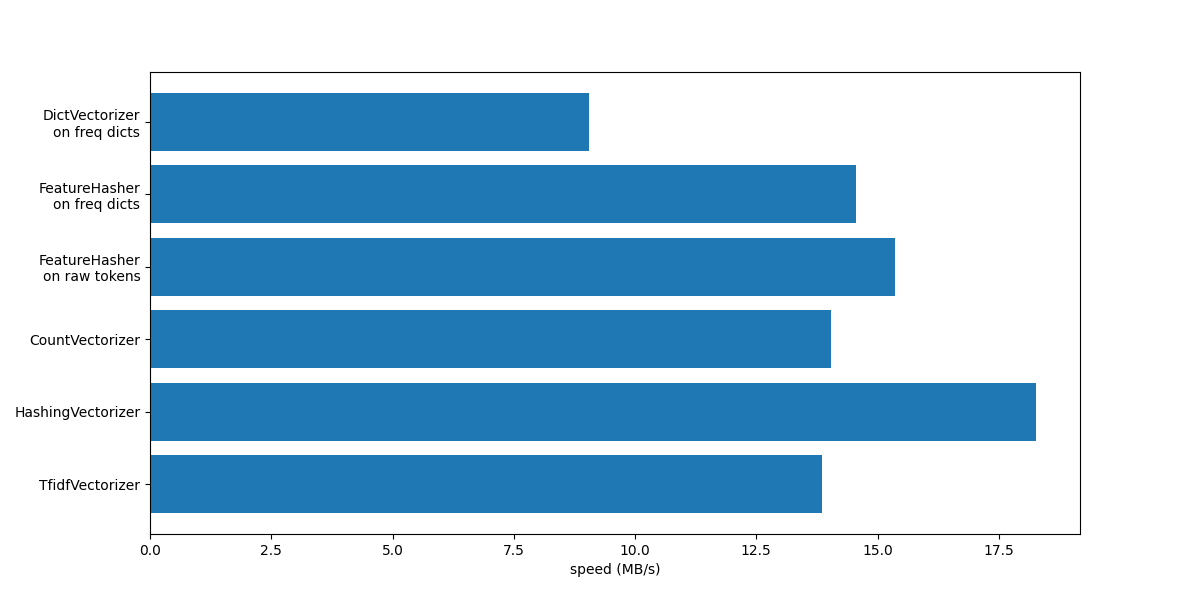
从图中可以看出, TfidfVectorizer 略慢于 CountVectorizer 由于 TfidfTransformer .
另请注意,通过设置功能数量 n_features = 2**18 , HashingVectorizer 表现比 CountVectorizer 代价是由于哈希冲突而导致转换的可逆性。
我们强调, CountVectorizer 和 HashingVectorizer 表现比同等产品更好 DictVectorizer 和 FeatureHasher 在手动标记化的文档上,因为以前的载体器的内部标记化步骤会编译一次正规表达,然后将其重新用于所有文档。
Total running time of the script: (0分3.554秒)
相关实例


Gallery generated by Sphinx-Gallery <https://sphinx-gallery.github.io> _