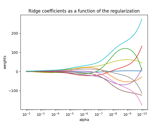
绘制岭系数作为正规化的函数#

显示估计量系数中共线性的影响。

Ridge 回归是本例中使用的估计量。每种颜色代表系数载体的不同特征，并且这显示为规则化参数的函数。

这个例子还展示了将岭回归应用于高度病态矩阵的有用性。对于此类矩阵，目标变量的轻微变化可能会导致计算权重的巨大差异。在这种情况下，设置一定的正规化（Alpha）以减少这种变化（噪音）是有用的。

当Alpha非常大时，规则化效应主导平方损失函数，并且系数趋于零。在路径的尽头，随着阿尔法趋于零，解趋于普通最小平方，系数就会表现出很大的波动。在实践中，有必要以保持两者之间的平衡的方式调整Alpha。

# Authors: The scikit-learn developers
# SPDX-License-Identifier: BSD-3-Clause

import matplotlib.pyplot as plt
import numpy as np

from sklearn import linear_model

# X is the 10x10 Hilbert matrix
X = 1.0 / (np.arange(1, 11) + np.arange(0, 10)[:, np.newaxis])
y = np.ones(10)

计算路径#

n_alphas = 200
alphas = np.logspace(-10, -2, n_alphas)

coefs = []
for a in alphas:
    ridge = linear_model.Ridge(alpha=a, fit_intercept=False)
    ridge.fit(X, y)
    coefs.append(ridge.coef_)

显示结果#

ax = plt.gca()

ax.plot(alphas, coefs)
ax.set_xscale("log")
ax.set_xlim(ax.get_xlim()[::-1])  # reverse axis
plt.xlabel("alpha")
plt.ylabel("weights")
plt.title("Ridge coefficients as a function of the regularization")
plt.axis("tight")
plt.show()