机器学习无法推断因果效应#

机器学习模型非常适合测量统计关联。不幸的是，除非我们愿意对数据做出强有力的假设，否则这些模型无法推断因果影响。

为了说明这一点，我们将模拟一种情况，在这种情况下，我们试图回答教育经济学中最重要的问题之一： what is the causal effect of earning a college degree on hourly wages? 尽管这个问题的答案对政策制定者至关重要， Omitted-Variable Biases (OVB)阻止我们识别这种因果效应。

# Authors: The scikit-learn developers
# SPDX-License-Identifier: BSD-3-Clause

数据集：模拟时薪#

数据生成过程在下面的代码中列出。工作经验（以年为单位）和能力指标来自正态分布;父母之一的小时工资来自贝塔分布。然后，我们创建了一个大学学位的指标，这是积极影响的能力和父母的时薪。最后，我们将小时工资建模为所有先前变量和随机分量的线性函数。请注意，所有变量对小时工资都有积极影响。

import numpy as np
import pandas as pd

n_samples = 10_000
rng = np.random.RandomState(32)

experiences = rng.normal(20, 10, size=n_samples).astype(int)
experiences[experiences < 0] = 0
abilities = rng.normal(0, 0.15, size=n_samples)
parent_hourly_wages = 50 * rng.beta(2, 8, size=n_samples)
parent_hourly_wages[parent_hourly_wages < 0] = 0
college_degrees = (
    9 * abilities + 0.02 * parent_hourly_wages + rng.randn(n_samples) > 0.7
).astype(int)

true_coef = pd.Series(
    {
        "college degree": 2.0,
        "ability": 5.0,
        "experience": 0.2,
        "parent hourly wage": 1.0,
    }
)
hourly_wages = (
    true_coef["experience"] * experiences
    + true_coef["parent hourly wage"] * parent_hourly_wages
    + true_coef["college degree"] * college_degrees
    + true_coef["ability"] * abilities
    + rng.normal(0, 1, size=n_samples)
)

hourly_wages[hourly_wages < 0] = 0

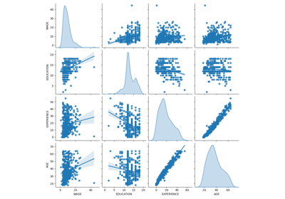
模拟数据的描述#

下图显示了每个变量的分布以及成对散点图。我们OVB故事的关键是能力和大学学位之间的正相关关系。

import seaborn as sns

df = pd.DataFrame(
    {
        "college degree": college_degrees,
        "ability": abilities,
        "hourly wage": hourly_wages,
        "experience": experiences,
        "parent hourly wage": parent_hourly_wages,
    }
)

grid = sns.pairplot(df, diag_kind="kde", corner=True)

在下一部分中，我们训练预测模型，因此我们将目标列与多个特征分开，并将数据分成训练集和测试集。

from sklearn.model_selection import train_test_split

target_name = "hourly wage"
X, y = df.drop(columns=target_name), df[target_name]
X_train, X_test, y_train, y_test = train_test_split(X, y, test_size=0.2, random_state=0)

充分观察变量的收入预测#

首先，我们训练预测模型， LinearRegression 模型在这个实验中，我们假设真正的生成模型使用的所有变量都可用。

from sklearn.linear_model import LinearRegression
from sklearn.metrics import r2_score

features_names = ["experience", "parent hourly wage", "college degree", "ability"]

regressor_with_ability = LinearRegression()
regressor_with_ability.fit(X_train[features_names], y_train)
y_pred_with_ability = regressor_with_ability.predict(X_test[features_names])
R2_with_ability = r2_score(y_test, y_pred_with_ability)

print(f"R2 score with ability: {R2_with_ability:.3f}")

R2 score with ability: 0.975

该模型很好地预测了小时工资，如高R2评分所示。我们绘制模型系数以表明我们准确地恢复了真实生成模型的值。

import matplotlib.pyplot as plt

model_coef = pd.Series(regressor_with_ability.coef_, index=features_names)
coef = pd.concat(
    [true_coef[features_names], model_coef],
    keys=["Coefficients of true generative model", "Model coefficients"],
    axis=1,
)
ax = coef.plot.barh()
ax.set_xlabel("Coefficient values")
ax.set_title("Coefficients of the linear regression including the ability features")
_ = plt.tight_layout()

Coefficients of the linear regression including the ability features

部分观测的收入预测#

在实践中，智力能力不会被观察到或仅通过无意中衡量教育程度的代理来估计（例如通过智商测试）。但从线性模型中省略“能力”特征会通过积极的OVB来扩大估计。

features_names = ["experience", "parent hourly wage", "college degree"]

regressor_without_ability = LinearRegression()
regressor_without_ability.fit(X_train[features_names], y_train)
y_pred_without_ability = regressor_without_ability.predict(X_test[features_names])
R2_without_ability = r2_score(y_test, y_pred_without_ability)

print(f"R2 score without ability: {R2_without_ability:.3f}")

R2 score without ability: 0.968

当我们省略R2分数方面的能力特征时，我们模型的预测能力是相似的。我们现在检查模型的系数是否与真正的生成模型不同。

model_coef = pd.Series(regressor_without_ability.coef_, index=features_names)
coef = pd.concat(
    [true_coef[features_names], model_coef],
    keys=["Coefficients of true generative model", "Model coefficients"],
    axis=1,
)
ax = coef.plot.barh()
ax.set_xlabel("Coefficient values")
_ = ax.set_title("Coefficients of the linear regression excluding the ability feature")
plt.tight_layout()
plt.show()

Coefficients of the linear regression excluding the ability feature

为了补偿省略的变量，该模型膨胀了大学学位特征的系数。因此，将此系数值解释为真正生成模型的因果效应是不正确的。

经验教训#

机器学习模型不是为了估计因果效应而设计的。虽然我们用线性模型展示了这一点，但OVB可以影响任何类型的模型。

每当解释一个系数或由一个特征的变化所带来的预测变化时，重要的是要记住潜在的未观察到的变量，这些变量可能与所讨论的特征和目标变量都相关。这些变量称为 Confounding Variables .为了在存在混淆的情况下仍然估计因果效应，研究人员通常会进行随机化治疗变量（例如大学学位）的实验。当实验成本过高或不道德时，研究人员有时可以使用其他因果推理技术，例如 Instrumental Variables (IV)估计。

Total running time of the script: （0分1.505秒）