变异Bayesian高斯混合物的浓度先验型分析

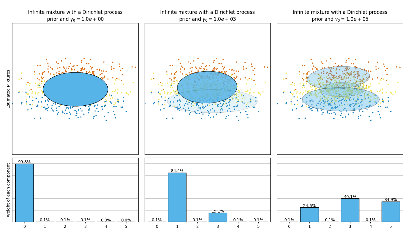
此示例绘制了从玩具数据集（三个高斯的混合）中获得的椭圆体，该数据集由 BayesianGaussianMixture 一类Dirichlet分布先验模型 (weight_concentration_prior_type='dirichlet_distribution' ）和Dirichlet过程之前 (weight_concentration_prior_type='dirichlet_process' ).在每张图上，我们绘制了之前重量浓度的三个不同值的结果。

的 BayesianGaussianMixture 类可以自动调整其混合成分的数量。参数 weight_concentration_prior 与所得到的具有非零权重的分量的数量有直接联系。如果浓度先验值较低，则模型会将大部分权重放在少数组分上，将其余组分的权重设置为非常接近于零。浓度先验的高值将允许更大数量的组分在混合物中具有活性。

Dirichlet流程previous允许定义无限数量的组件并自动选择正确数量的组件：仅在必要时才会激活组件。

相反，具有Dirichlet分布先验的经典有限混合模型将有利于更均匀的加权分量，因此倾向于将自然集群划分为不必要的子分量。

• 
• 

# Authors: The scikit-learn developers
# SPDX-License-Identifier: BSD-3-Clause

import matplotlib as mpl
import matplotlib.gridspec as gridspec
import matplotlib.pyplot as plt
import numpy as np

from sklearn.mixture import BayesianGaussianMixture


def plot_ellipses(ax, weights, means, covars):
    for n in range(means.shape[0]):
        eig_vals, eig_vecs = np.linalg.eigh(covars[n])
        unit_eig_vec = eig_vecs[0] / np.linalg.norm(eig_vecs[0])
        angle = np.arctan2(unit_eig_vec[1], unit_eig_vec[0])
        # Ellipse needs degrees
        angle = 180 * angle / np.pi
        # eigenvector normalization
        eig_vals = 2 * np.sqrt(2) * np.sqrt(eig_vals)
        ell = mpl.patches.Ellipse(
            means[n], eig_vals[0], eig_vals[1], angle=180 + angle, edgecolor="black"
        )
        ell.set_clip_box(ax.bbox)
        ell.set_alpha(weights[n])
        ell.set_facecolor("#56B4E9")
        ax.add_artist(ell)


def plot_results(ax1, ax2, estimator, X, y, title, plot_title=False):
    ax1.set_title(title)
    ax1.scatter(X[:, 0], X[:, 1], s=5, marker="o", color=colors[y], alpha=0.8)
    ax1.set_xlim(-2.0, 2.0)
    ax1.set_ylim(-3.0, 3.0)
    ax1.set_xticks(())
    ax1.set_yticks(())
    plot_ellipses(ax1, estimator.weights_, estimator.means_, estimator.covariances_)

    ax2.get_xaxis().set_tick_params(direction="out")
    ax2.yaxis.grid(True, alpha=0.7)
    for k, w in enumerate(estimator.weights_):
        ax2.bar(
            k,
            w,
            width=0.9,
            color="#56B4E9",
            zorder=3,
            align="center",
            edgecolor="black",
        )
        ax2.text(k, w + 0.007, "%.1f%%" % (w * 100.0), horizontalalignment="center")
    ax2.set_xlim(-0.6, 2 * n_components - 0.4)
    ax2.set_ylim(0.0, 1.1)
    ax2.tick_params(axis="y", which="both", left=False, right=False, labelleft=False)
    ax2.tick_params(axis="x", which="both", top=False)

    if plot_title:
        ax1.set_ylabel("Estimated Mixtures")
        ax2.set_ylabel("Weight of each component")


# Parameters of the dataset
random_state, n_components, n_features = 2, 3, 2
colors = np.array(["#0072B2", "#F0E442", "#D55E00"])

covars = np.array(
    [[[0.7, 0.0], [0.0, 0.1]], [[0.5, 0.0], [0.0, 0.1]], [[0.5, 0.0], [0.0, 0.1]]]
)
samples = np.array([200, 500, 200])
means = np.array([[0.0, -0.70], [0.0, 0.0], [0.0, 0.70]])

# mean_precision_prior= 0.8 to minimize the influence of the prior
estimators = [
    (
        "Finite mixture with a Dirichlet distribution\n" r"prior and $\gamma_0=$",
        BayesianGaussianMixture(
            weight_concentration_prior_type="dirichlet_distribution",
            n_components=2 * n_components,
            reg_covar=0,
            init_params="random",
            max_iter=1500,
            mean_precision_prior=0.8,
            random_state=random_state,
        ),
        [0.001, 1, 1000],
    ),
    (
        "Infinite mixture with a Dirichlet process\n" r"prior and $\gamma_0=$",
        BayesianGaussianMixture(
            weight_concentration_prior_type="dirichlet_process",
            n_components=2 * n_components,
            reg_covar=0,
            init_params="random",
            max_iter=1500,
            mean_precision_prior=0.8,
            random_state=random_state,
        ),
        [1, 1000, 100000],
    ),
]

# Generate data
rng = np.random.RandomState(random_state)
X = np.vstack(
    [
        rng.multivariate_normal(means[j], covars[j], samples[j])
        for j in range(n_components)
    ]
)
y = np.concatenate([np.full(samples[j], j, dtype=int) for j in range(n_components)])

# Plot results in two different figures
for title, estimator, concentrations_prior in estimators:
    plt.figure(figsize=(4.7 * 3, 8))
    plt.subplots_adjust(
        bottom=0.04, top=0.90, hspace=0.05, wspace=0.05, left=0.03, right=0.99
    )

    gs = gridspec.GridSpec(3, len(concentrations_prior))
    for k, concentration in enumerate(concentrations_prior):
        estimator.weight_concentration_prior = concentration
        estimator.fit(X)
        plot_results(
            plt.subplot(gs[0:2, k]),
            plt.subplot(gs[2, k]),
            estimator,
            X,
            y,
            r"%s$%.1e$" % (title, concentration),
            plot_title=k == 0,
        )

plt.show()

相关实例

高斯混合模型顺曲线

Gaussian Mixture Model Sine Curve

高斯混合模型椭圆体

Gaussian Mixture Model Ellipsoids

高斯混合物的密度估计

Density Estimation for a Gaussian mixture

邻里要素分析插图

Neighborhood Components Analysis Illustration