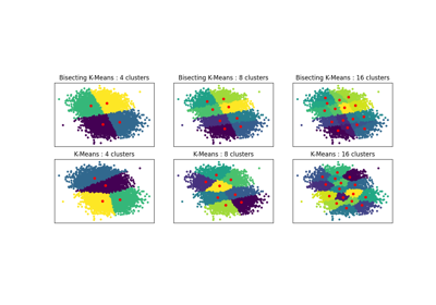
备注
Go to the end 下载完整的示例代码。或者通过浏览器中的MysterLite或Binder运行此示例
在KMeans聚类中使用轮廓分析选择聚类数#
剪影分析可用于研究所得集群之间的分离距离。轮廓图显示一个集群中的每个点与邻近集群中的点的接近程度的测量,从而提供了一种视觉评估集群数量等参数的方法。该措施有一系列 [-1, 1] .
接近+1的剪影系数(这些值称为)表示样本远离邻近集群。值为0表示样本位于或非常接近两个相邻集群之间的决策边界,负值表示这些样本可能被分配给错误的集群。
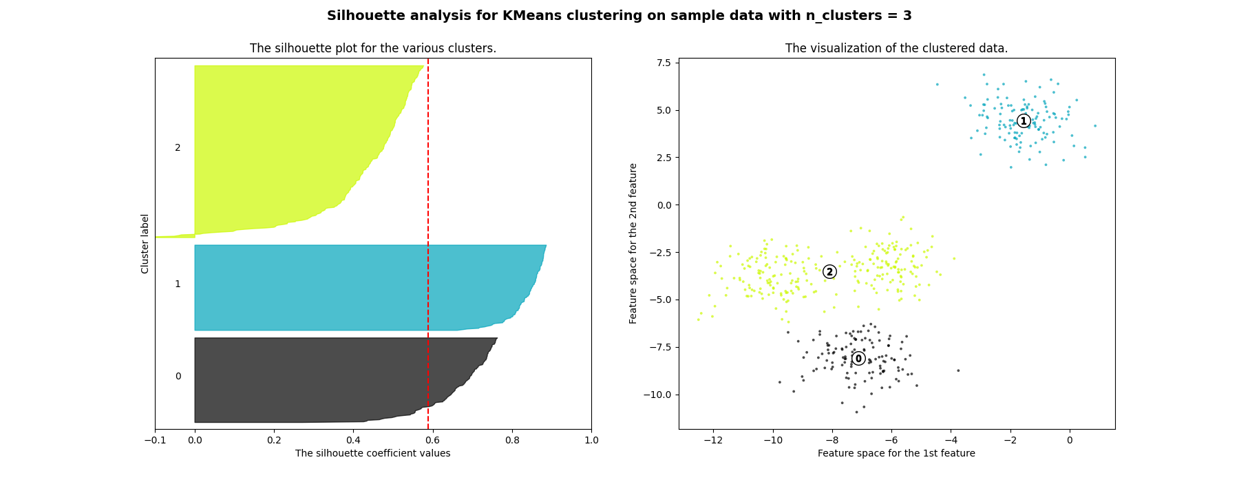
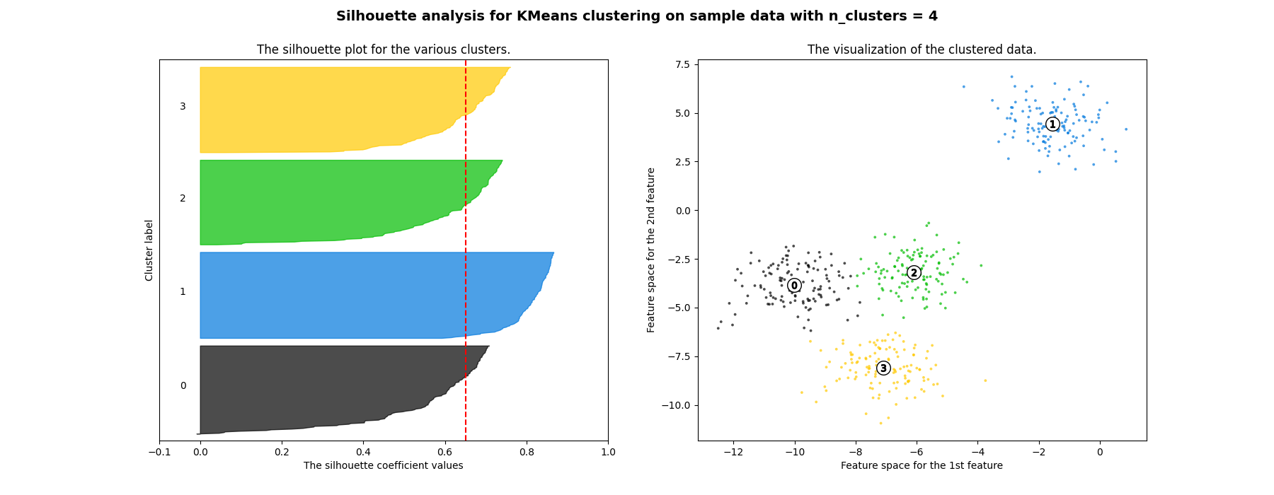
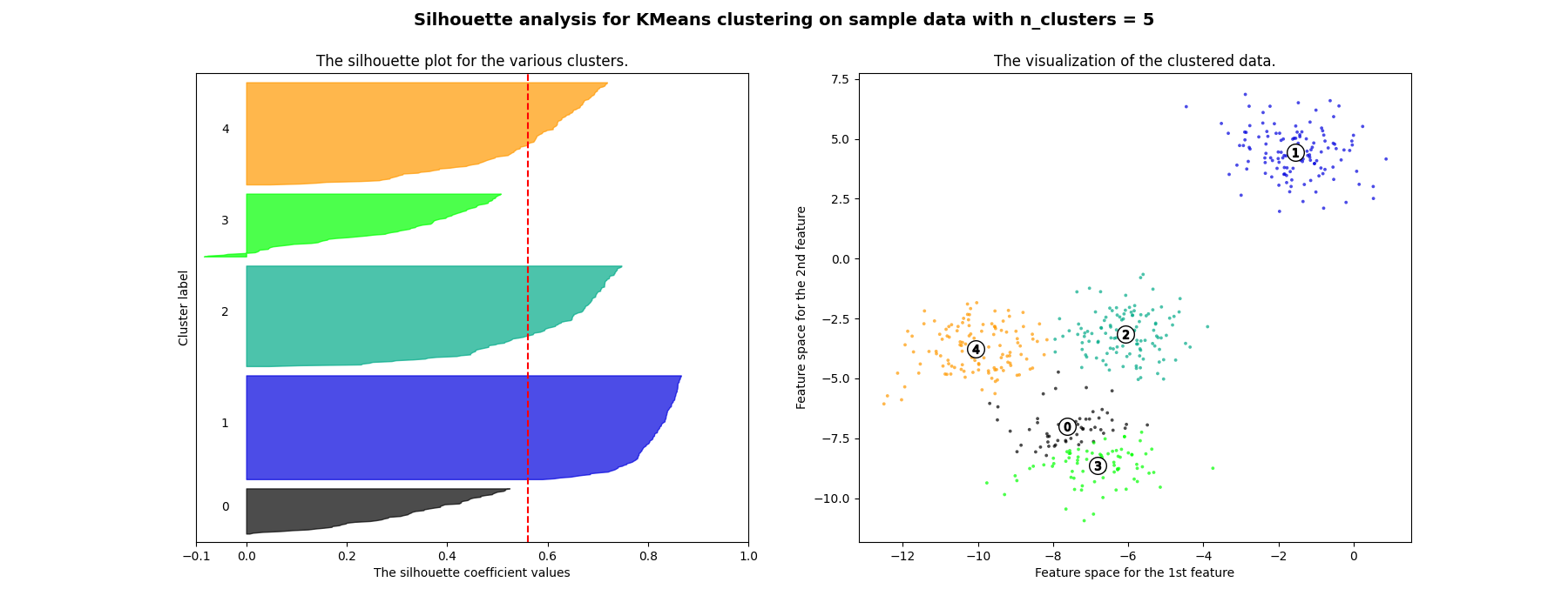
在本例中,使用轮廓分析来选择最佳值, n_clusters .剪影情节表明 n_clusters 对于给定数据来说,值3、5和6是一个糟糕的选择,因为存在具有低于平均轮廓分数的集群,并且还因为轮廓图的大小波动很大。剪影分析在2和4之间做出决定时更加矛盾。
此外,从轮廓图的厚度可以可视化集群大小。当情况下,群0的轮廓图 n_clusters 等于2,由于将3个子集群分组为一个大集群,因此大小更大。然而当 n_clusters 等于4,则所有图的厚度或多或少相似,因此具有相似的大小,这也可以从右侧标记的散点图中验证。
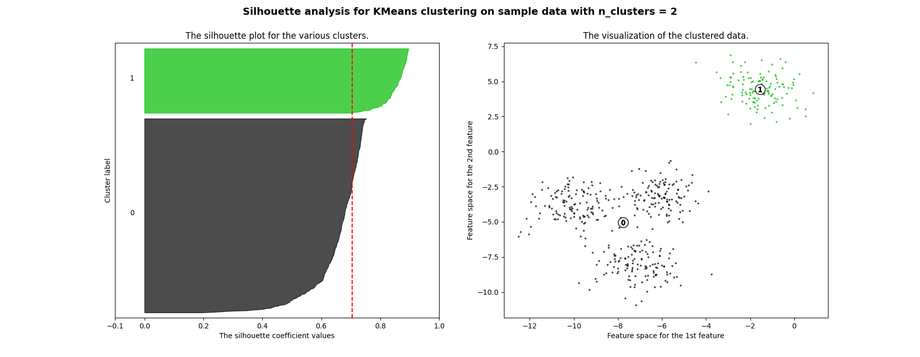

For n_clusters = 2 The average silhouette_score is : 0.7049787496083262
For n_clusters = 3 The average silhouette_score is : 0.5882004012129721
For n_clusters = 4 The average silhouette_score is : 0.6505186632729437
For n_clusters = 5 The average silhouette_score is : 0.561464362648773
For n_clusters = 6 The average silhouette_score is : 0.4857596147013469
# Authors: The scikit-learn developers
# SPDX-License-Identifier: BSD-3-Clause
import matplotlib.cm as cm
import matplotlib.pyplot as plt
import numpy as np
from sklearn.cluster import KMeans
from sklearn.datasets import make_blobs
from sklearn.metrics import silhouette_samples, silhouette_score
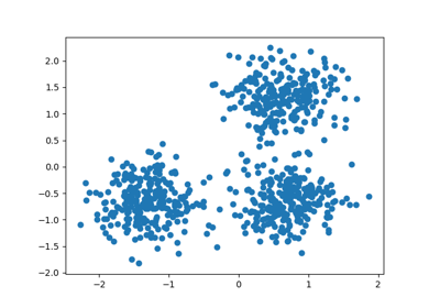
# Generating the sample data from make_blobs
# This particular setting has one distinct cluster and 3 clusters placed close
# together.
X, y = make_blobs(
n_samples=500,
n_features=2,
centers=4,
cluster_std=1,
center_box=(-10.0, 10.0),
shuffle=True,
random_state=1,
) # For reproducibility
range_n_clusters = [2, 3, 4, 5, 6]
for n_clusters in range_n_clusters:
# Create a subplot with 1 row and 2 columns
fig, (ax1, ax2) = plt.subplots(1, 2)
fig.set_size_inches(18, 7)
# The 1st subplot is the silhouette plot
# The silhouette coefficient can range from -1, 1 but in this example all
# lie within [-0.1, 1]
ax1.set_xlim([-0.1, 1])
# The (n_clusters+1)*10 is for inserting blank space between silhouette
# plots of individual clusters, to demarcate them clearly.
ax1.set_ylim([0, len(X) + (n_clusters + 1) * 10])
# Initialize the clusterer with n_clusters value and a random generator
# seed of 10 for reproducibility.
clusterer = KMeans(n_clusters=n_clusters, random_state=10)
cluster_labels = clusterer.fit_predict(X)
# The silhouette_score gives the average value for all the samples.
# This gives a perspective into the density and separation of the formed
# clusters
silhouette_avg = silhouette_score(X, cluster_labels)
print(
"For n_clusters =",
n_clusters,
"The average silhouette_score is :",
silhouette_avg,
)
# Compute the silhouette scores for each sample
sample_silhouette_values = silhouette_samples(X, cluster_labels)
y_lower = 10
for i in range(n_clusters):
# Aggregate the silhouette scores for samples belonging to
# cluster i, and sort them
ith_cluster_silhouette_values = sample_silhouette_values[cluster_labels == i]
ith_cluster_silhouette_values.sort()
size_cluster_i = ith_cluster_silhouette_values.shape[0]
y_upper = y_lower + size_cluster_i
color = cm.nipy_spectral(float(i) / n_clusters)
ax1.fill_betweenx(
np.arange(y_lower, y_upper),
0,
ith_cluster_silhouette_values,
facecolor=color,
edgecolor=color,
alpha=0.7,
)
# Label the silhouette plots with their cluster numbers at the middle
ax1.text(-0.05, y_lower + 0.5 * size_cluster_i, str(i))
# Compute the new y_lower for next plot
y_lower = y_upper + 10 # 10 for the 0 samples
ax1.set_title("The silhouette plot for the various clusters.")
ax1.set_xlabel("The silhouette coefficient values")
ax1.set_ylabel("Cluster label")
# The vertical line for average silhouette score of all the values
ax1.axvline(x=silhouette_avg, color="red", linestyle="--")
ax1.set_yticks([]) # Clear the yaxis labels / ticks
ax1.set_xticks([-0.1, 0, 0.2, 0.4, 0.6, 0.8, 1])
# 2nd Plot showing the actual clusters formed
colors = cm.nipy_spectral(cluster_labels.astype(float) / n_clusters)
ax2.scatter(
X[:, 0], X[:, 1], marker=".", s=30, lw=0, alpha=0.7, c=colors, edgecolor="k"
)
# Labeling the clusters
centers = clusterer.cluster_centers_
# Draw white circles at cluster centers
ax2.scatter(
centers[:, 0],
centers[:, 1],
marker="o",
c="white",
alpha=1,
s=200,
edgecolor="k",
)
for i, c in enumerate(centers):
ax2.scatter(c[0], c[1], marker="$%d$" % i, alpha=1, s=50, edgecolor="k")
ax2.set_title("The visualization of the clustered data.")
ax2.set_xlabel("Feature space for the 1st feature")
ax2.set_ylabel("Feature space for the 2nd feature")
plt.suptitle(
"Silhouette analysis for KMeans clustering on sample data with n_clusters = %d"
% n_clusters,
fontsize=14,
fontweight="bold",
)
plt.show()
Total running time of the script: (0分0.863秒)
相关实例

Gallery generated by Sphinx-Gallery <https://sphinx-gallery.github.io> _